Matmul (Multi Core)
We’ll build a program that will perform matmul operations on two tensors with equal-size inner dimension on as many cores as possible on the accelerator. This example builds on top of the previous single core matmul example.
In terms of API usage, there isn’t much change. We will discuss the specific changes to:
Distribute the work across multiple cores.
Set up each core to process a subset of the tiles.
What changes (and what doesn’t change) in the API usage to achieve this.
It is important to note that this example builds on top of the previous single core matmul example, so it is recommended to understand the single core matmul example first. The single core matmul example is available under the tt_metal/programming_examples/matmul_single_core/ directory.
The full source code for this example is available under the tt_metal/programming_examples/matmul/matmul_multi_core/ directory.
Building the example can be done by adding a --build-programming-examples flag to the build script or adding the -DBUILD_PROGRAMMING_EXAMPLES=ON flag to the cmake command and results in the metal_example_matmul_multi_core executable in the build/programming_examples directory. For example:
export TT_METAL_HOME=</path/to/tt-metal>
./build_metal.sh --build-programming-examples
./build/programming_examples/metal_example_matmul_multi_core
Note
Efficiently parallelizing matrix multiplication across multiple cores—using SPMD (Single Program, Multiple Data) or other parallelization strategies - is a broad and advanced topic, often covered in depth in advanced computer science courses. While this tutorial demonstrates how to use our API to distribute work across cores, it does not attempt to teach the fundamentals of parallel programming or SPMD concepts themselves.
If you are new to these topics, we recommend consulting external resources or textbooks on parallel computing for a deeper understanding. This will help you make the most of our platform and adapt these examples to your own use cases.
For further reading on parallel programming and SPMD, see the References section at the end of this document.
Device Initialization & Program Setup
Device initialization and parameter setup are similar to the single core example, but now use the mesh API. You create a mesh device, initialize the program, and compute the reference result on the CPU. Example:
// Open mesh device (use device 0)
constexpr int device_id = 0;
auto mesh_device = distributed::MeshDevice::create_unit_mesh(device_id);

// Matrix dimensions (must be divisible by tile dimensions)
constexpr uint32_t M = 640;  // Matrix A height
constexpr uint32_t N = 640;  // Matrix B width
constexpr uint32_t K = 640;  // Shared dimension

// Calculate number of tiles in each dimension
uint32_t Mt = M / TILE_HEIGHT;  // Each tile is 32x32
uint32_t Kt = K / TILE_WIDTH;
uint32_t Nt = N / TILE_WIDTH;

std::mt19937 rng(std::random_device{}());
std::uniform_real_distribution<float> dist(-0.5f, 0.5f);

std::vector<bfloat16> src0_vec(M * K, 0);  // Matrix A (MxK)
std::vector<bfloat16> src1_vec(K * N, 0);  // Matrix B (KxN)
// Fill with random bfloat16 values
for (bfloat16& v : src0_vec) {
    v = bfloat16(dist(rng));
}
for (bfloat16& v : src1_vec) {
    v = bfloat16(dist(rng));
}

std::vector<bfloat16> golden_vec(M * N, 0);
golden_matmul(src0_vec, src1_vec, golden_vec, M, N, K);

// Convert source matrices to tiled format for device execution
src0_vec = tilize_nfaces(src0_vec, M, K);
src1_vec = tilize_nfaces(src1_vec, K, N);

// Set up mesh command queue, workload, and program
distributed::MeshCommandQueue& cq = mesh_device->mesh_command_queue();
distributed::MeshWorkload workload;
distributed::MeshCoordinateRange device_range = distributed::MeshCoordinateRange(mesh_device->shape());
Program program{};

// Create DRAM buffers for input and output matrices (replicated per device across the mesh)
constexpr uint32_t single_tile_size = sizeof(bfloat16) * TILE_HEIGHT * TILE_WIDTH;
distributed::DeviceLocalBufferConfig dram_config{
    .page_size = single_tile_size, .buffer_type = tt_metal::BufferType::DRAM};
distributed::ReplicatedBufferConfig buffer_config_A{.size = single_tile_size * Mt * Kt};
distributed::ReplicatedBufferConfig buffer_config_B{.size = single_tile_size * Nt * Kt};
distributed::ReplicatedBufferConfig buffer_config_C{.size = single_tile_size * Mt * Nt};

auto src0_dram_buffer = distributed::MeshBuffer::create(buffer_config_A, dram_config, mesh_device.get());
auto src1_dram_buffer = distributed::MeshBuffer::create(buffer_config_B, dram_config, mesh_device.get());
auto dst_dram_buffer = distributed::MeshBuffer::create(buffer_config_C, dram_config, mesh_device.get());
Next, convert the source matrices to tiled format before preparing for execution on the device.
src0_vec = tilize_nfaces(src0_vec, M, K);
src1_vec = tilize_nfaces(src1_vec, K, N);
Calculating Work Distribution
Tenstorrent’s AI processors support multiple parallelization strategies. The grid structure of the AI processors enables various approaches to distributing work. In this example, we use a simple SPMD (Single Program, Multiple Data) strategy similar to GPU programming. Each core runs the same program but processes a different subset of the data to compute the full result. We parallelize across the output tiles of the result matrix, with each core responsible for producing 1/num_cores of the output tiles, where num_cores is the number of available cores.
Note
The SPMD strategy is a standard approach in parallel computing and works well for many workloads. However, for matrix multiplication, the most efficient method on Tenstorrent’s AI processors is to use a systolic array pattern, and use a subset of cores to read in and reuse the read data. This example does not cover that approach. See Matmul (Multi Core Optimized) for further optimizations, at the cost of genericity. SPMD remains a flexible and general-purpose strategy, making it suitable for a variety of tasks in Metalium.
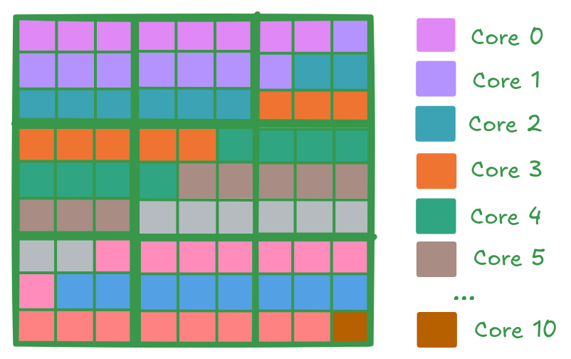
For a matrix of size 288 x 288 (9 tiles along each dimension, with each tile being 32x32), and 11 cores available, the work is divided as evenly as possible. In the example case, 10 cores are assigned 8 output tiles each, and the 11th core processes the remaining tile. The diagram below shows how the output tiles are distributed among the cores. Each color corresponds to a different core, and each tile is handled by only one core:
Metalium includes utilities to simplify work distribution across cores. The tt::tt_metal::split_work_to_cores(core_grid, num_work) function calculates how many tiles each core should process, based on the total amount of work and the number of available cores. It distributes the work as evenly as possible, even if the number of tiles does not divide evenly among the cores. The function returns several values:
num_cores: Number of cores used for the operation.all_cores: Set of all cores assigned to the operation.core_group_1: Primary group of cores, each handling more work.core_group_2: Secondary group of cores, each handling less work (empty if the work divides evenly).work_per_core1: Number of output tiles each core in the primary group processes.work_per_core2: Number of output tiles each core in the secondary group processes (0 if the work divides evenly).
For example, if you need to split 81 output tiles across 11 cores, split_work_to_cores may distribute the work as follows:
num_cores= 11 (all 11 cores are used)all_cores= all 11 corescore_group_1= first 10 cores (each processes 8 tiles)core_group_2= last core (processes 1 tile)work_per_core1= 8 (tiles per core in the primary group)work_per_core2= 1 (tiles for the secondary group core)
auto core_grid = device->compute_with_storage_grid_size();
uint32_t num_output_tiles = (M * N) / TILE_HW; // number of output tiles

auto [num_cores, all_cores, core_group_1, core_group_2, work_per_core1, work_per_core2] =
    tt::tt_metal::split_work_to_cores(core_grid, num_output_tiles);
Note
The following properties describe the output of tt::tt_metal::split_work_to_cores:
all_coresis the set of cores assigned work for this operation.If there is not enough work,
all_coresmay be smaller than the total number of cores incore_grid.all_corescontains exactlynum_corescores.all_coresis always the union ofcore_group_1andcore_group_2.The total amount of work (
num_work) is always fully assigned:work_per_core1 * num_cores_in_core_group_1 + work_per_core2 * num_cores_in_core_group_2 == num_work.The function automatically handles uneven work distribution; you do not need to manage edge cases manually.
Note
How Metalium Parallelism Differs from OpenCL/CUDA
In frameworks like OpenCL and CUDA, you typically launch many more work groups (or thread blocks) than there are physical compute units. The hardware scheduler dynamically assigns these work groups to available compute units. If a group of threads (warp/wavefront) stalls - such as waiting for memory - the scheduler can quickly switch to another ready group, keeping the hardware busy and improving overall throughput. This dynamic scheduling and oversubscription allow for automatic load balancing and efficient handling of workloads with unpredictable execution times.
In contrast, Metalium’s parallelism model is static. The number of parallel tasks you can launch is limited to the number of available Tensix cores on the device. Each core is assigned a specific portion of the work at launch, and there is no dynamic scheduling or oversubscription: once a core finishes its assigned work, it remains idle until the next task is launched. This is similar to static scheduling in OpenMP, where work is divided as evenly as possible among available threads at the start.
As a result, when using Metalium, it is important to:
Carefully partition your workload so that all cores are kept busy.
Be aware that you cannot launch more tasks than there are cores.
Understand that dynamic load balancing (as in CUDA/OpenCL) is not available.
This model offers predictable performance and is well-suited for workloads that can be evenly distributed, but it requires more attention to work distribution for optimal efficiency.
Buffer and Circular Buffer Allocation
Creating buffers and circular buffers in Metalium is similar to the single core example. For circular buffers, instead of creating them on a single core, you create them on all cores that will be used in the operation.
// Allocate DRAM buffers (shared resources on the device). Nothing changes here.
constexpr uint32_t single_tile_size = sizeof(bfloat16) * TILE_HEIGHT * TILE_WIDTH;
auto src0_dram_buffer = CreateBuffer({
    .device = device,
    .size = single_tile_size * Mt * Kt,
    .page_size = single_tile_size,
    .buffer_type = tt_metal::BufferType::DRAM
});
auto src1_dram_buffer = CreateBuffer({
    .device = device,
    .size = single_tile_size * Nt * Kt,
    .page_size = single_tile_size,
    .buffer_type = tt_metal::BufferType::DRAM
});
auto dst_dram_buffer = CreateBuffer({
    .device = device,
    .size = single_tile_size,
    .page_size = single_tile_size,
    .buffer_type = tt_metal::BufferType::DRAM
});

// Create circular buffers on all participating cores
const auto cb_data_format = tt::DataFormat::Float16_b;
uint32_t num_input_tiles = 2;
auto cb_src0 = tt_metal::CreateCircularBuffer(
    program, all_cores, // create on all cores
    CircularBufferConfig(num_input_tiles * single_tile_size, {{CBIndex::c_0, cb_data_format}})
        .set_page_size(CBIndex::c_0, single_tile_size)
);

auto cb_src1 = tt_metal::CreateCircularBuffer(
    program, all_cores, // create on all cores
    CircularBufferConfig(num_input_tiles * single_tile_size, {{CBIndex::c_1, cb_data_format}})
        .set_page_size(CBIndex::c_1, single_tile_size)
);

auto cb_output = tt_metal::CreateCircularBuffer(
    program, all_cores, // create on all cores
    CircularBufferConfig(num_input_tiles * single_tile_size, {{CBIndex::c_16, cb_data_format}})
        .set_page_size(CBIndex::c_16, single_tile_size)
);
Partitioning Work in Kernels
To support work distribution, the kernel is updated so that each core processes only its assigned portion of the output. Instead of having one core handle the entire matrix, we add parameters to the kernel that specify how many tiles each core should process and the starting tile index. This way, each core computes a subset of the output tiles. Below is the writer kernel, which writes the output tiles to the DRAM buffer:
void kernel_main() {
    uint32_t dst_addr = get_arg_val<uint32_t>(0);
    uint32_t num_tiles = get_arg_val<uint32_t>(1); // Number of tiles to write
    uint32_t start_id = get_arg_val<uint32_t>(2);  // Starting tile ID for this core

    constexpr uint32_t cb_id_out = tt::CBIndex::c_16;

    const uint32_t tile_bytes = get_tile_size(cb_id_out);

    constexpr auto c_args = TensorAccessorArgs<0>();
    const auto c = TensorAccessor(c_args, dst_addr, tile_bytes);

    // Each core writes only its assigned tiles
    for (uint32_t i = 0; i < num_tiles; ++i) {
        cb_wait_front(cb_id_out, 1);
        uint32_t l1_read_addr = get_read_ptr(cb_id_out);
        // Write to the correct offset based on start_id
        noc_async_write_page(i + start_id, c, l1_read_addr);
        noc_async_write_barrier();
        cb_pop_front(cb_id_out, 1);
    }
}
The compute kernel does not handle IO directly and is not concerned with how work is distributed among the cores. It only needs to know how many tiles to compute and the size of the inner dimension. The kernel is almost identical to the single core version, except that the number of tiles to process is passed as a parameter:
void kernel_main() {
    uint32_t num_output_tiles = get_arg_val<uint32_t>(0); // Number of output tiles to produce
    uint32_t Kt = get_arg_val<uint32_t>(1); // Size of the inner dimension (K)

    constexpr tt::CBIndex cb_in0 = tt::CBIndex::c_0;
    constexpr tt::CBIndex cb_in1 = tt::CBIndex::c_1;
    constexpr tt::CBIndex cb_out = tt::CBIndex::c_16;

    mm_init(cb_in0, cb_in1, cb_out);

    // Instead of processing all tiles, we process only the assigned amount of tiles.
    for (uint32_t i = 0; i < num_output_tiles; ++i) {
        tile_regs_acquire();
        // Same inner loop as in the single core example, only the outer loop is adjusted
        // to produce the assigned number of tiles.
        for (uint32_t kt = 0; kt < Kt; kt++) {
            cb_wait_front(cb_in0, 1);
            cb_wait_front(cb_in1, 1);

            matmul_tiles(cb_in0, cb_in1, 0, 0, 0);

            cb_pop_front(cb_in0, 1);
            cb_pop_front(cb_in1, 1);
        }

        tile_regs_commit();
        tile_regs_wait();

        cb_reserve_back(cb_out, 1);
        pack_tile(0, cb_out);
        cb_push_back(cb_out, 1);

        tile_regs_release();
    }
}
The reader kernel is responsible for reading the input data from the DRAM buffers and pushing it into the circular buffers. It also needs to know how many tiles to read and the starting tile index for each core. Due to needing to calculate where to start reading from the DRAM buffer, it also needs to know the exact dimensions of the input matrices (Mt, Kt, Nt). Again the reader is almost identical to the single core version, except that it reads only the assigned number of tiles and uses the starting tile index to calculate the correct offset in the DRAM buffer:
void kernel_main() {
    uint32_t src0_addr = get_arg_val<uint32_t>(0);
    uint32_t src1_addr = get_arg_val<uint32_t>(1);
    uint32_t Mt = get_arg_val<uint32_t>(2);
    uint32_t Kt = get_arg_val<uint32_t>(3);
    uint32_t Nt = get_arg_val<uint32_t>(4);
    uint32_t output_tile_start_id = get_arg_val<uint32_t>(5); // Starting tile ID for this core
    uint32_t num_output_tiles = get_arg_val<uint32_t>(6); // Number of output tiles to read

    constexpr uint32_t cb_id_in0 = tt::CBIndex::c_0;
    constexpr uint32_t cb_id_in1 = tt::CBIndex::c_1;

    const uint32_t in0_tile_bytes = get_tile_size(cb_id_in0);
    const uint32_t in1_tile_bytes = get_tile_size(cb_id_in1);

    constexpr auto a_args = TensorAccessorArgs<0>();
    const auto a = TensorAccessor(a_args, src0_addr, in0_tile_bytes);

    constexpr auto b_args = TensorAccessorArgs<a_args.next_compile_time_args_offset()>();
    const auto b = TensorAccessor(b_args, src1_addr, in1_tile_bytes);

    // Loop through the output tiles assigned to this core
    for (uint32_t output_tile = 0; output_tile < num_output_tiles; output_tile++) {
        uint32_t current_tile_id = output_tile_start_id + output_tile;

        // Calculate the output tile position in the grid
        uint32_t out_row = current_tile_id / Nt;
        uint32_t out_col = current_tile_id % Nt;

        // Read all K tiles for this output position. Same inner loop as in the single core example.
        for (uint32_t k = 0; k < Kt; k++) {
            uint32_t tile_A = out_row * Kt + k;
            {
                cb_reserve_back(cb_id_in0, 1);
                uint32_t l1_write_addr_in0     = get_write_ptr(cb_id_in0);
                noc_async_read_page(tile_A, a, l1_write_addr_in0);
                noc_async_read_barrier();
                cb_push_back(cb_id_in0, 1);
            }

            uint32_t tile_B = k * Nt + out_col;
            {
                cb_reserve_back(cb_id_in1, 1);
                uint32_t l1_write_addr_in1 = get_write_ptr(cb_id_in1);
                noc_async_read_page(tile_B, b, l1_write_addr_in1);
                noc_async_read_barrier();
                cb_push_back(cb_id_in1, 1);
            }
        }
    }
}
Kernel Creation and Parameter Setup
With the work distribution calculated, you can now create the kernels and set up their parameters. Since not all cores may be used, make sure to create kernels only on the cores listed in all_cores. This avoids having idle kernels on unused cores.
Warning
If a kernel is created on a core but runtime arguments are not set for that core, the program may crash or hang as a result of undefined behavior. Always ensure that kernels are created only on the intended cores, or that runtime arguments are set for every core where a kernel is created.
MathFidelity math_fidelity = MathFidelity::HiFi4;  // High fidelity math for accurate results
std::vector<uint32_t> reader_compile_time_args;
TensorAccessorArgs(*src0_dram_buffer).append_to(reader_compile_time_args);
TensorAccessorArgs(*src1_dram_buffer).append_to(reader_compile_time_args);
auto reader_id = tt_metal::CreateKernel(
    program,
    OVERRIDE_KERNEL_PREFIX "matmul/matmul_multi_core/kernels/dataflow/reader_mm_output_tiles_partitioned.cpp",
    all_cores,
    tt_metal::DataMovementConfig{
        .processor = DataMovementProcessor::RISCV_1,
        .noc = NOC::RISCV_1_default,
        .compile_args = reader_compile_time_args});

std::vector<uint32_t> writer_compile_time_args;
TensorAccessorArgs(*dst_dram_buffer).append_to(writer_compile_time_args);
auto writer_id = tt_metal::CreateKernel(
    program,
    OVERRIDE_KERNEL_PREFIX "matmul/matmul_multi_core/kernels/dataflow/writer_unary_interleaved_start_id.cpp",
    all_cores,
    tt_metal::DataMovementConfig{
        .processor = DataMovementProcessor::RISCV_0,
        .noc = NOC::RISCV_0_default,
        .compile_args = writer_compile_time_args});

auto compute_kernel_id = tt_metal::CreateKernel(
    program,
    OVERRIDE_KERNEL_PREFIX "matmul/matmul_multi_core/kernels/compute/mm.cpp",
    all_cores,
    tt_metal::ComputeConfig{.math_fidelity = math_fidelity, .compile_args = {}});
Unlike OpenCL or CUDA, Metalium does not provide built-in parameters for work distribution on the device. You need to manually set the runtime arguments for each core. This is done by iterating through the work groups and assigning the correct arguments for each core, including buffer addresses, tile counts, and the amount of work assigned.
uint32_t work_offset = 0;
auto work_groups = {
    std::make_pair(core_group_1, work_per_core1), std::make_pair(core_group_2, work_per_core2)};

// Iterate through each work group and assign work to cores
for (const auto& [ranges, work_per_core] : work_groups) {
    // Each core group may be formed of multiple ranges, so we iterate
    // through each range (splitting up 2D grid may result in fragmented ranges)
    for (const auto& range : ranges.ranges()) {
        // For each core in the range, set the runtime arguments for the
        // reader, writer, and compute kernels
        for (const auto& core : range) {
            // Set arguments for the reader kernel (data input)
            tt_metal::SetRuntimeArgs(
                program,
                reader_id,
                core,
                {src0_dram_buffer->address(),
                 src1_dram_buffer->address(),
                 Mt,
                 Kt,
                 Nt,
                 work_offset,                  // Starting offset for this core's work
                 work_per_core});              // Amount of work for this core

            // Set arguments for the writer kernel (data output)
            tt_metal::SetRuntimeArgs(
                program, writer_id, core, {dst_dram_buffer->address(),
                work_per_core,                 // Amount of work for this core
                work_offset});                 // Starting offset for this core's work

            // Set arguments for the compute kernel
            tt_metal::SetRuntimeArgs(
                program,
                compute_kernel_id,
                core,
                {work_per_core,            // Amount of work for this core
                 Kt});
            work_offset += work_per_core;  // Update offset for next core
        }
    }
}
Program Execution, Receiving Results and Cleanup
This part is the same as in the single core example. You execute the program, wait for it to finish, and then download the results from the DRAM buffer. The cleanup process is also unchanged.
See Kernel execution and result verification in the single core matrix multiplication in the single core matrix multiplication example for details on how program execution, downloading results, untilize, verification, and cleanup are performed. There is no change in the API usage for these steps compared to the single core example.
// Upload input data to DRAM buffers using mesh API
distributed::EnqueueWriteMeshBuffer(cq, src0_dram_buffer, a, false);
distributed::EnqueueWriteMeshBuffer(cq, src1_dram_buffer, b, false);

// Add program to mesh workload and execute
workload.add_program(device_range, std::move(program));
distributed::EnqueueMeshWorkload(cq, workload, false);

// Download results from DRAM buffer to host
distributed::EnqueueReadMeshBuffer(cq, output, dst_dram_buffer, true);

// outside of the function, `output` is returned as `result_vec`
result_vec = untilize_nfaces(result_vec, M, N);


float pearson = check_bfloat16_vector_pcc(golden_vec, result_vec);
log_info(tt::LogVerif, "Metalium vs Golden -- PCC = {}", pearson);
TT_FATAL(pearson > 0.97, "PCC not high enough. Result PCC: {}, Expected PCC: 0.97", pearson);

// Properly close the mesh device to release resources
mesh_device->close();
Conclusion
This concludes the multi-core matmul example and the basic usage of the Metalium API to distribute work across multiple cores. The key changes compared to the single core example are:
Work distribution calculations using the
tt::tt_metal::split_work_to_coresfunctionAllocate circular buffers across all cores that will be used in the operation
Set runtime arguments for each core to specify how many tiles to process and the starting tile index
Adjust the kernels to process only the assigned number of tiles and use the starting tile index for reading/writing data
Create kernels on the cores that will be used in the operation and handle edge cases like uneven work distribution or fewer cores than work
Explore Matmul (Multi Core Optimized) for further optimizations, including data reuse and data multicast to truly harness the power of the Tenstorrent architecture.
References
For those interested in learning more about parallel programming concepts, we recommend the following resources:
Intel OpenMP Tutorial — A comprehensive YouTube series covering OpenMP as well as fundamental parallel programming concepts.
A “Hands-On” Introduction to OpenMP — A detailed PDF guide that provides a practical introduction to OpenMP, which is a widely used API for parallel programming in C/C++ and Fortran.