What to Know About Your Workstation

Your workstation is a Tenstorrent Quietbox 2: four AI accelerators inside, an operating system you may not have used before, and the software stack already configured and waiting. The machine is ready to go — what’s left is knowing what you’ve got.

This guide doesn’t assume you know Linux, or Python, or what a PCIe slot is. It assumes you’re curious, and that curiosity is enough.

What’s Inside

The Tenstorrent Quietbox 2 (QB2) is a workstation with two Blackhole p300c cards — four Blackhole chips in total — on PCIe. Each p300c is a dual-chip card, and each chip is independent — four separate devices from the software’s point of view, connected to a standard CPU running Ubuntu 24.04 LTS.

The chips don’t share memory. When you open device 0, you’re talking to one Blackhole chip. To use all four together, you use ttnn.CreateDevices({0, 1, 2, 3}) — not four separate open_device() calls.

What Ships Pre-Installed

Tenstorrent ships the QB2 ready to serve models. You don’t install drivers. You don’t compile anything. The full stack is already there:

• Kernel driver — loaded automatically at boot, makes the chips visible to software
• tt-smi — hardware monitoring tool, lives at /usr/bin/tt-smi
• TTNN Python environment — pre-built venv at ~/tt-metal/python_env/
• vLLM — in the main tenstorrent venv at ~/.tenstorrent-venv/
• TT-Forge/XLA — container wrapper at ~/.local/bin/tt-forge
• tt-studio — the no-code web UI for serving models, pre-installed (launch with tt-studio)
• A ready-to-run model — Qwen3-32B, weights pre-cached on disk, deployable from tt-studio with no download
• Firmware — already flashed to all four chips

What’s intentionally absent: the ~/tt-metal source code. The environments are there; the source isn’t. You can build models, run inference, and work with the full API stack without it. Building from source is a later chapter — a much later chapter.

Physical Tour

The QB2 looks like a standard tower workstation. On the inside:

• CPU and motherboard running Ubuntu 24.04 LTS
• Two Blackhole p300c cards (four Blackhole chips total)
• RAM sized for production inference workloads
• Storage for model weights — but watch it carefully (more on that in Chapter 2)

The chips run warm under load. Fans will get louder when you run inference. This is correct. The cooling is designed for sustained operation at full chip temperature.

One Blackhole chip. You have four, on two p300c cards.

Next: First Boot →

First Boot

Power on. Ubuntu loads. You log in. Now what?

Everything from here happens in a terminal. That’s the command line — a text window where you type instructions and the machine responds. On a QB2, the terminal is your instrument panel. Learning its three or four most-used commands will get you surprisingly far.

Finding a Terminal

If you’re looking at the GNOME desktop:

• Press Ctrl+Alt+T — opens a terminal on most Ubuntu setups
• Or press the Super key (Windows key), type terminal, press Enter
• Or right-click the desktop and choose “Open Terminal”

Once a terminal window is open, you’re in the right place. It shows a prompt ending in $ — everything you type goes after that.

The Three Commands You Need Right Now

Check disk space first. Models are large. This is non-negotiable to understand before you do anything else:

df -h ~

This shows your home directory’s disk usage. The Size column is total, Avail is what’s free. You need room — at minimum 3 GB for a small model (Qwen3-0.6B), 20+ GB for anything like Llama-3.1-8B. If you’re under 5 GB free, stop here and figure out where the space went before continuing.

Check internet connectivity:

ping -c 3 google.com

If this fails, check your network cable or go to Settings → Network. Everything else in this guide requires internet access for model downloads.

Update the package list (do this once after first boot):

sudo apt update

sudo means “run as administrator.” Ubuntu will ask for your password. This doesn’t install or change anything — it just refreshes the list of what’s available. You’ll see a lot of text scroll by. That’s normal.

Ubuntu: What You Should Know

The QB2 runs Ubuntu 24.04 LTS. If this is your first time with it:

• Package manager is apt — install things with sudo apt install <name>
• Files are case-sensitive: Model.py and model.py are different files
• Your home directory is ~ — short for /home/yourusername
• sudo runs a command as administrator — use it only when a command tells you to

Your Login, Password, and SSH

Many QB2 units ship with a default login — username ttuser, password ttuser. If that’s how yours arrived, change the password the moment you’re in, before the machine is reachable on a shared network:

passwd

It asks for the current password (ttuser), then a new one twice.

Turn on SSH

Later in this guide — and on every other path — you reach the QB2 from your own laptop over SSH: forwarding a model server’s port back to your machine, copying files, running commands remotely. SSH isn’t always running on a fresh box, so turn it on once:

# Install and enable the SSH server
sudo apt install -y openssh-server
sudo systemctl enable --now ssh

# Confirm it's listening
systemctl status ssh

Then find the address other machines use to reach you:

hostname -I     # the QB2's IP address on your network
hostname        # its name — often <name>.local

From your laptop you can now run ssh ttuser@<that-ip>. This is what makes the remote-access steps in Serving Models on QB2 — and bringing tt-studio’s web UI to your own browser — work.

Python: A Field Guide to the Confusion

This is where new Linux users often hit a wall. Ubuntu ships with its own Python. The Tenstorrent software has its own Python environments. These are separate and don’t mix. Here’s the landscape:

What exists on your system

Why does this matter?

Ubuntu 24.04 enforces what’s called externally-managed Python — the system Python is protected. If you try to pip install something directly, Ubuntu will refuse with an error about breaking system packages. This is intentional. It protects you.

The right move is always: activate the correct venv, then install inside it. The Tenstorrent venvs already have everything you need for this guide, so you won’t need to install much.

What which python3 tells you

Before running any Python code, check which Python is active:

which python3

If you see /usr/bin/python3 — you’re using the system Python. Tenstorrent imports will fail.

If you see something like /home/yourname/tt-metal/python_env/bin/python3 — you’re inside the right venv. Go ahead.

pip, pyenv, uv — a brief map

You may encounter other Python tools in documentation or online:

• pip — Python package installer. Works inside a venv. Fine to use there.
• pyenv — manages multiple Python versions (3.10, 3.11, etc.). The QB2 doesn’t need it — the venvs handle version isolation.
• virtualenv / python -m venv — creates isolated environments. The Tenstorrent venvs were built this way.
• uv — a fast, modern alternative to pip and virtualenv. Works, but the QB2 docs and this guide use standard venv activation.

For this guide: ignore pyenv, ignore uv. Activate the venv Tenstorrent provides. That’s all you need.

Activating and deactivating

# Activate the TTNN environment
source ~/tt-metal/python_env/bin/activate

# Your prompt now shows (python_env) — you're inside
# Deactivate when done
deactivate

The (python_env) prefix in your prompt is the signal. When it’s there, Python calls and imports go to the right place. When it’s not, they don’t.

Next: Is This Thing On? →

Is This Thing On?

Before running a model, confirm the hardware is alive and the software can see it. One command, four chips, zero guessing.

Reading Your Hardware with tt-smi

tt-smi is the Tenstorrent System Management Interface. Your window into the chips. Run it in snapshot mode to get JSON instead of the interactive TUI:

tt-smi -s

A healthy QB2 returns four entries — one per Blackhole chip:

{
  "device_info": [
    {
      "board_type": "BLACKHOLE",
      "board_id": "AA-BHXY-0001",
      "pcie_speed": "GEN4",
      "pcie_width": "x16",
      "temperature": { "asic": 44.1, "inlet": 31.0 },
      "voltage": { "core": 0.85 },
      "power": { "total": 42.0 }
    }
  ]
}

Four entries in device_info means four chips, all alive. Check it directly:

tt-smi -s | python3 -m json.tool | grep board_type

You should see "BLACKHOLE" printed four times.

Reading the Output

A healthy QB2 shows four entries in device_info. Look at each one for:

• "board_type": "BLACKHOLE" — confirms chip family. If you see anything else, something’s wrong.
• "pcie_speed": "GEN4" — PCIe link is up at full speed. GEN3 would mean a slot compatibility issue.
• "pcie_width": "x16" — full-width link. Narrower means lower bandwidth.
• Temperature in the 35–55°C range — normal at idle. Higher under load is fine.

Count the entries:

tt-smi -s | python3 -c "import sys,json; d=json.load(sys.stdin); print(len(d['device_info']), 'devices')"

If you see 4 devices, move on. The QB2 is ready.

If You See Fewer Than Four

A missing device usually means one of three things:

PCIe link not established:

dmesg | grep -i tenstorrent | tail -20

Look for errors about PCIe enumeration or firmware loading failure. A loose card is possible — the QB2 ships with cards seated, but transit happens.

Firmware mismatch:

tt-smi -s | python3 -m json.tool | grep -i fw_version

If firmware versions differ across devices, or show 0.0.0, you may need to reflash. See the tt-flash documentation for instructions.

Driver not loaded:

lsmod | grep tenstorrent

If nothing prints, the kernel driver isn’t loaded. This shouldn’t happen on a stock QB2, but if it does:

sudo modprobe tenstorrent

Watching in Real Time

For a live view of all four chips while running inference:

tt-smi

This opens the interactive TUI — press q to quit. You’ll see per-chip utilization, temperature, and memory usage update live. Useful when a model is running and you want to see all four chips light up.

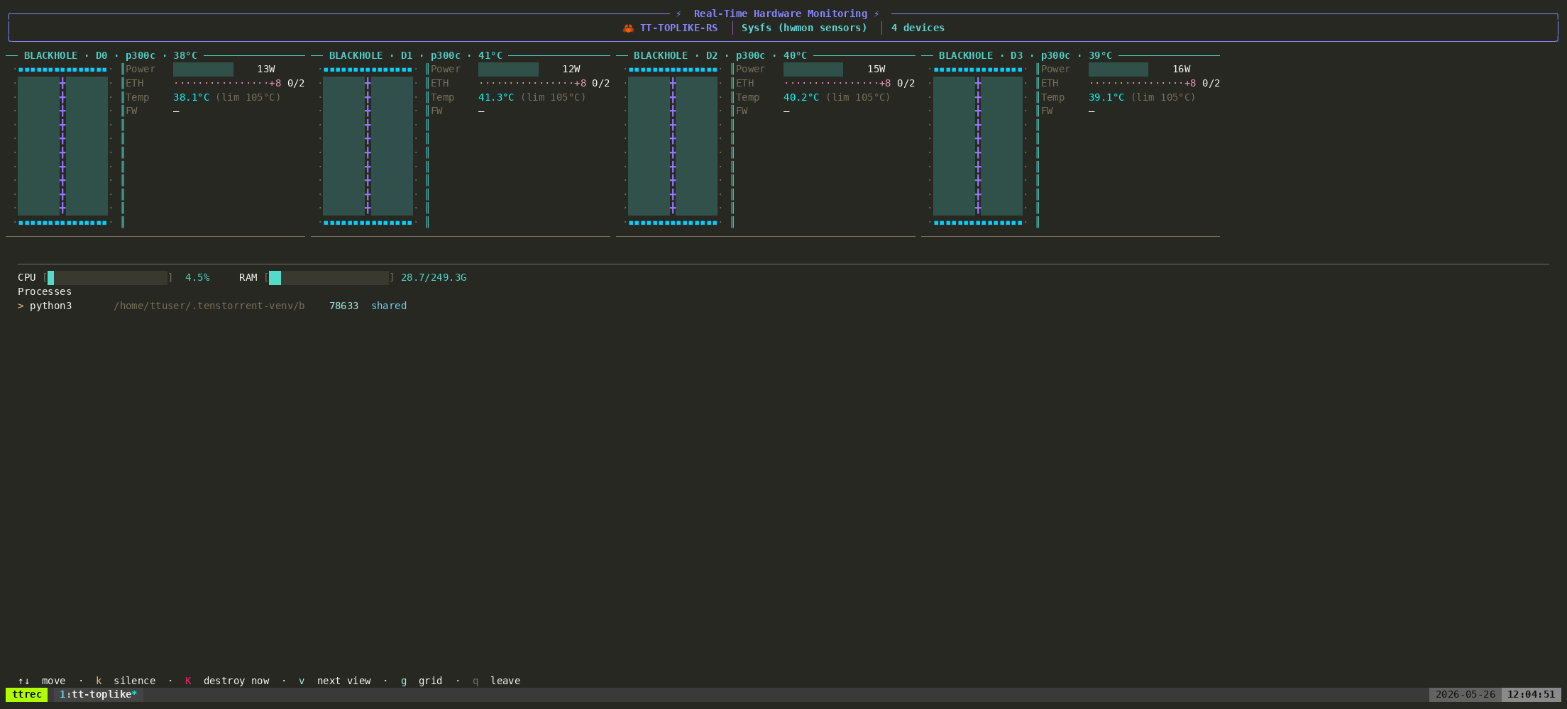
For something richer than the built-in TUI, tt-toplike renders the same telemetry as live ASCII art — every chip’s power, temperature, and DRAM state, animated:

This is what active inference looks like inside one chip. Four of these run in parallel on a QB2.

Next: Installing the Stack →

Installing the Stack

On a QB2 from Tenstorrent, this is already done. The venvs are there, the driver is loaded, the firmware is flashed. This chapter is for understanding what exists and where — so you know which environment to activate when, and what to do if something’s missing.

Installing the Tenstorrent Software Stack

On a QB2 from Tenstorrent, the stack is already there. This section is for installing on a fresh Ubuntu system, or understanding what the installer put where.

Prerequisites: Ubuntu 24.04 LTS (or 22.04), internet connection, sudo access.

sudo apt update && sudo apt install -y curl jq
/bin/bash -c "$(curl -fsSL https://github.com/tenstorrent/tt-installer/releases/latest/download/install.sh)"

The installer handles drivers, firmware, kernel modules, and all three Python environments. Accept the defaults — they’re right for a QB2.

After it finishes, reboot:

sudo reboot

What ends up on your QB2

As of tt-installer v3.2.0, Docker is the default container runtime (Podman is still supported — pass --install-container-runtime=podman). The Metalium container installs by default. Forge is not installed by default — the TT-Forge docs install it as a pip wheel (pip install pjrt-plugin-tt … then tt-forge-install); tt-installer’s --install-forge-container is an optional convenience, not the recommended path. See the TT-Forge chapter for the full install. On a QB2 that shipped from Tenstorrent, the TTNN venv at ~/tt-metal/python_env/ is pre-built. The ~/tt-metal/ directory contains compiled environments — not the tt-metal source code.

What You Have

On a QB2 from Tenstorrent, the stack is pre-installed. Here’s your map:

Create the scratch directory if it doesn’t exist yet:

mkdir -p ~/tt-scratchpad ~/models

The Three Environments, Explained

TTNN (~/tt-metal/python_env/)

This is the workhorse. Use it for direct Python API work — opening devices, running TTNN operations, the cookbook examples in this guide.

source ~/tt-metal/python_env/bin/activate
# prompt changes to (python_env)
python3 -c "import ttnn; print('TTNN ready')"
deactivate

vLLM (in ~/.tenstorrent-venv)

Use this to run a model as a server with an OpenAI-compatible HTTP API. vLLM is available in the main tenstorrent venv:

source ~/.tenstorrent-venv/bin/activate
vllm serve ~/models/Qwen3-0.6B --port 8000

Or use tt-studio for a no-code UI that handles vLLM startup automatically.

TT-Forge — install it yourself with pip

Unlike TTNN and vLLM, Forge is not something a stock install hands you. The TT-Forge docs install it as a pip wheel into a Python 3.12 venv — TT-XLA is the frontend for PyTorch and JAX:

source ~/.tenstorrent-venv/bin/activate
pip install pjrt-plugin-tt --extra-index-url https://pypi.eng.aws.tenstorrent.com/
tt-forge-install

Models then compile via torch.compile(model, backend="tt") (PyTorch) or jax.jit (JAX). Prebuilt Docker images and an ONNX frontend exist too — the TT-Forge chapter has the full walkthrough.

Confirming Each Environment Works

Run this check sequence:

# TTNN
source ~/tt-metal/python_env/bin/activate
python3 -c "import ttnn; print('✓ TTNN')" && deactivate

# vLLM (in the main tenstorrent venv)
source ~/.tenstorrent-venv/bin/activate
python3 -c "import vllm; print('✓ vLLM')" && deactivate

# Check for the tt-smi binary
which tt-smi && tt-smi --version

All three should respond without errors. If TTNN import fails, the venv may not be set up — check docs.tenstorrent.com for the current setup guide. If tt-smi isn’t found, add ~/.local/bin to your PATH (see below).

Installing tt-smi if it’s Missing

On a QB2 it shouldn’t be missing, but on another Ubuntu system:

# Option A — public PyPI (any machine, no PPA needed):
pip install tt-smi

# Option B — via apt (requires Tenstorrent PPA, set up by tt-installer):
sudo apt install tt-smi

Both install the same tool. Option A works anywhere with Python; option B integrates with your system package manager. On a freshly installed Ubuntu machine without tt-installer, option A is the easier path.

Disk Space and Model Storage

Models consume significant disk space. Plan accordingly:

The convention across all Tenstorrent documentation is ~/models/<model-name>/. Nothing enforces this — you can store models anywhere and point --model at any path — but using the convention means every tutorial command works without substitution.

Check space before any download:

df -h ~/models

Next: Your First Model →

Your First Model

Everything up to now was preparation. This is the part where the machine does something interesting. Four chips, waiting. One small model, about to arrive.

Running Your First Model

This chapter takes the other path — the hands-on one, where you talk to a chip directly in Python and pull a tiny model down yourself. The starter is Qwen/Qwen3-0.6B — no license gate, 1.5 GB, runs on any Tenstorrent hardware.

First, activate the TTNN environment and verify the hardware is accessible:

source ~/tt-metal/python_env/bin/activate

Your prompt will change to show (python_env). That which python3 will now point into the venv, not /usr/bin/python3. Check it:

which python3
# → /home/yourname/tt-metal/python_env/bin/python3

Now do the handshake — open a device, confirm it responds, close it:

python3 -c "
import ttnn
device = ttnn.open_device(device_id=0)
print('Device open:', device)
ttnn.close_device(device)
print('Done.')
"

If you see Device open: without errors, chip 0 is alive and responding. Repeat with device_id=1, 2, 3 to verify all four.

Download a model

Use the hf CLI (part of the huggingface_hub package already installed in the venv):

# hf — not huggingface-cli. The command is hf.
hf download Qwen/Qwen3-0.6B --local-dir ~/models/Qwen3-0.6B

This creates ~/models/Qwen3-0.6B/ with the HuggingFace-format weights (~1.5 GB). Check your disk first:

df -h ~

You need at least 3 GB free for this model alone. Larger models (Llama-3.1-8B) need 16+ GB.

What Just Happened

When that Python snippet ran without errors, the Blackhole chip opened a dispatch channel through the PCIe link, initialized its RISC-V cores, and confirmed it can receive work. Nothing computed yet. But the handshake — software to silicon — is the prerequisite for everything else.

ttnn.open_device(0) — what happens inside the chip.

Serving a Model with vLLM

The fastest path to actually generating text is vLLM. It handles model loading, tokenization, batching, and presents an OpenAI-compatible HTTP API.

source ~/.tenstorrent-venv/bin/activate

# Make sure the model is downloaded first (see above)
# Then start the server:
python3 -m vllm.entrypoints.openai.api_server \
  --model ~/models/Qwen3-0.6B \
  --port 8000

You’ll see initialization messages as the model loads. This takes a minute or two on first run — the model weights are being compiled for the Blackhole architecture. Subsequent runs are faster.

Once you see INFO: Application startup complete, the server is ready. In a new terminal:

curl -s http://localhost:8000/v1/chat/completions \
  -H "Content-Type: application/json" \
  -d '{
    "model": "Qwen3-0.6B",
    "messages": [{"role": "user", "content": "What makes the Tenstorrent Blackhole chip different?"}]
  }' | python3 -m json.tool

The response is JSON. The answer is in choices[0].message.content.

Using tt-studio (the Web UI)

tt-studio

tt-studio is a web interface for running models on QB2 without writing a line of code. It handles model selection, container lifecycle, and inference end-to-end — open a browser, pick a model, get tokens back.

Start it with a single command on the QB2:

tt-studio

Then open http://localhost:3000 in your browser, pick a model from the Deploy Model dropdown, and click Run. On a QB2, Qwen3-32B is already there with its weights pre-cached — its first deploy skips the multi-GB download and is ready in a few minutes. Other models download on first use; after that, every run loads fast from the on-disk cache.

What’s happening under the hood: tt-studio is a UI sitting on top of tt-inference-server. When you select a model and click Run, tt-studio spins up a Docker container running the TT fork of vLLM on port 8000. Your browser talks to tt-studio; tt-studio talks to that container. tt-local-generator routes through the same container — both are UIs sitting on top of tt-inference-server, just with different front ends.

To access tt-studio from your laptop while the QB2 is on your network, forward the port over SSH:

ssh -L 3000:localhost:3000 user@qb2-hostname

Then open http://localhost:3000 on your local machine as if you were sitting in front of the QB2.

For a deeper look at how the inference server is wired up, the tt-vscode-toolkit lesson on tt-inference-server walks through the architecture interactively — Docker flags, model download, port mapping, and what logs to watch on first boot.

Multi-Device: Using All Four Chips

To spread a model across all four Blackhole chips, use CreateDevices instead of open_device:

source ~/tt-metal/python_env/bin/activate

python3 -c "
import ttnn
devices = ttnn.CreateDevices({0, 1, 2, 3})
print('All devices:', devices)
ttnn.CloseDevices(devices)
print('Done.')
"

CreateDevices handles the mesh configuration that lets the chips coordinate. Models loaded this way can distribute layers across chips, increasing the effective memory pool and throughput. Large models (Llama-3.1-70B) require this — they don’t fit on one chip’s memory alone.

CreateDevices spans all four chips: a large model's layers spread across them for more memory and throughput. (A small model like Qwen3-0.6B runs happily on one chip.)

Next: What Comes Next →

What Comes Next

You unboxed a machine that most people have never touched. You confirmed four Blackhole chips were alive and talking to the system. You navigated Python environments that would trip up someone who wasn’t paying attention. You ran a model on accelerator hardware and watched tokens come back. That’s not a tutorial warmup — that’s the actual thing.

The rest is up to you.

Tools in Your World

The QB2 ships with a full stack, but the ecosystem is bigger. Start with tt-toplike — htop for your chips, except the telemetry comes alive as ASCII art:

Where to Go From Here

Pick a thing you want to do and jump straight in.

Choose Your Next Track

The QB2 is a beginning. There’s a lot of surface area here, and you’ve only scratched it.

← Back to Explore

Coming From CUDA

You know cudaMalloc. You know grid-dim and block-dim. You’ve tuned shared memory usage, you’ve written custom CUDA kernels, and you’ve debugged timing issues with Nsight. You have a mental model of how GPU compute actually works, not just how PyTorch wraps it.

That mental model transfers here, but not intact. Some pieces map cleanly. Some don’t exist. And some things you were papering over on the GPU are now explicit, visible, and tunable. The next ten minutes remaps the terrain.

Pick Your Altitude

The first question a CUDA developer asks is “where’s my model.cuda()?” The honest answer is that there isn’t one entry point — there are three, and which one you reach for depends on how much control you want. CUDA has the same three tiers; you just rarely think about them as a stack because NVIDIA blurs the seams.

The closest thing to model.cuda() is the top tier: TT-Forge traces your graph and lowers it to Tensix automatically. That’s Chapter 6 — reach for it when you want the model to just run. The two bottom tiers are for the cases TTNN doesn’t cover: TT-Lang lets you write a custom kernel in Python with no C++, and TT-Metalium is the C++ floor where every abstraction disappears. Both live in the Builder/Hacker track — and, as the last section of this chapter explains, the TT-Lang tier is far more reachable than “write your own kernel” sounds on CUDA.

This track lives in the middle, at TTNN — the tier where you have hand-optimized ops but still write Python, not kernels. It’s the sweet spot for performance work that doesn’t require descending to the metal, so that’s where the rest of this chapter focuses.

Thread Blocks vs. Tensix Tiles

On a GPU, a thread block is the unit of cooperative work: a group of threads that can share L1/shared memory and synchronize. The programmer launches a grid of blocks; the hardware schedules them onto SMs.

On Blackhole, the unit is a Tensix core. There are 120 enabled per chip (a 12×10 block of the 14×10 physical Tensix grid), sitting inside a larger 17×12 NoC grid that also carries DRAM, Ethernet, and PCIe nodes. Each core has its own L1 SRAM, its own set of RISC-V processing cores (five of them), and its own connection to the Network-on-Chip (NoC) fabric that threads through the entire grid. Tensix cores don’t share memory with each other. There’s no “block-scope” shared memory. There’s only what one core holds, and what it explicitly sends over the NoC to another.

This is the fundamental shift. On CUDA, data sharing between threads in a block is cheap and implicit — shared memory just works. On Tensix, data movement is the thing you design around. Every byte a core receives came from somewhere specific, via a routed packet on the NoC. That movement is visible to you. It’s also where the performance is.

There’s a deeper reason it’s visible: there is no warp scheduler hiding memory latency. On a GPU, when one warp stalls waiting on a global-memory read, the SM scheduler instantly swaps in another resident warp — latency disappears behind oversubscription, and you mostly don’t think about it. Tensix has no such trick. Instead, each core runs an explicit reader → compute → writer pipeline: one RISC-V core streams tiles into L1, the matrix engine works on them, another core streams results out, and they overlap by design rather than by lucky scheduling. At the TTNN level you don’t write that pipeline — the ops do — but it’s why tensor layout matters so much here. A layout that lets the reader stage clean tiles keeps the pipeline full; one that forces a reshuffle stalls it, and there’s no spare warp to paper over the gap.

L1 SRAM vs. Shared Memory

Each Tensix core has 1.5 MB of L1 SRAM. On a GPU, your shared memory budget is typically 48–96 KB per SM, and you fight for it. On Tensix, you have a full 1.5 MB per core to work with.

The catch: that memory doesn’t auto-populate. On a GPU, you launch a kernel and global memory reads happen via caches. On Tensix, you write the code that moves data from DRAM (the rows at the top and bottom of the chip grid) into the L1 of whichever cores need it. TTNN does this for you when you use its built-in ops — but if you drop to Metalium, you’re writing those NoC reads yourself.

For someone writing at the TTNN Python level (which is where this track lives), the takeaway is simpler: tensor operations in TTNN are already written to stage data correctly. You don’t write data movement code. But you do care about tensor layout, because layout determines whether the underlying kernels can move data efficiently or have to reshuffle it first.

TTNN as the CUDA Runtime Equivalent

Think of TTNN the way you think of libcudart plus cuBLAS plus cuDNN — all fused into one Python API. It handles device open/close, tensor allocation in device memory, op dispatch, kernel compilation (via Metalium under the hood), and synchronization.

The critical difference from cuBLAS: TTNN compiles ops JIT on first invocation. When you run a matrix multiply for the first time on a new tensor shape, Metalium generates a Tensix kernel for that exact configuration. Subsequent calls with the same shape hit the op cache and run fast. This is why first-run latency can be a few seconds — and why subsequent runs are fast enough to serve production traffic.

import ttnn
import torch

# Open a single chip (device_id=0)
device = ttnn.open_device(device_id=0)

# Move a PyTorch tensor to device
torch_a = torch.randn(1024, 1024)
a = ttnn.from_torch(torch_a, device=device, dtype=ttnn.bfloat16)

# This compiles on first run, then caches
result = ttnn.matmul(a, a)

# Pull back to CPU
out = ttnn.to_torch(result)
ttnn.close_device(device)

Compare this to CUDA: cudaMemcpy, cublasSgemm, cudaMemcpy back. The pattern is the same. The surface is different.

What Transfers From CUDA Knowledge

Tensor shapes, batch dimensions, attention head patterns — all of this maps directly. The math doesn’t change. The numerics don’t change (bfloat16 is first-class here, same as modern GPUs). Batching strategies that work on GPU work on Tensix.

Knowledge of kernel fusion matters. The same principle applies: fewer round-trips through memory means faster execution. TTNN has fused ops (fused attention, fused feedforward) that follow the same logic as FlashAttention on CUDA.

Multi-device tensor parallelism maps directly too. The QB2 has four chips. When you run a 70B model, attention heads get split across chips the same way they’d split across GPUs in a tensor-parallel setup. The API is different — ttnn.CreateDevices({0,1,2,3}) instead of torch.distributed — but the concept transfers.

What Doesn’t Transfer

CUBLAS and cuDNN don’t exist here. There’s no drop-in replacement. If your code calls torch.nn.functional.conv2d and you want it to run on Blackhole, you need to either use TTNN’s conv2d op or compile via TT-Forge (which traces PyTorch graphs and lowers them to TTNN). You can’t just model.cuda() and move on.

Device memory pointers are gone. CUDA lets you grab a raw void* to device memory and pass it around. TTNN tensors are opaque objects — no raw pointer access. If your code does custom CUDA pointer arithmetic, that approach doesn’t port. You use TTNN ops, or you write Metalium kernels (a Tinker track topic).

Unified memory has no equivalent. There’s no cudaMallocManaged. Data is either on CPU or on the device, and you move it explicitly via ttnn.from_torch and ttnn.to_torch.

Grid launch syntax is gone. There’s no <<<gridDim, blockDim>>>. Kernel dispatch is handled by the TTNN op, which decides how to tile the work across the Tensix grid. You influence this via tensor layout and op selection, not by choosing block/thread dimensions.

CUDA Concept Mapping Table

Blackhole’s NoC Fabric

The four Blackhole chips in your QB2 sit on two p300c cards, linked by Warp cables and on-chip Ethernet — not PCIe (PCIe is only the host-to-card link). Intra-chip, the NoC connects every core to every other core and to the DRAM banks at roughly 1 TB/s aggregate bandwidth. This is not the same topology as NVLink or PCIe between discrete GPUs — it’s a different architecture where the cost of moving data within a chip is much lower relative to compute throughput than on a GPU.

For multi-chip workloads, the four chips form a mesh using their Ethernet cores (the left and right columns of the chip grid). This is how tensor-parallel models distribute their KV-cache updates — not through the host CPU, but directly chip-to-chip.

Matrix multiply: DRAM rows stage the operand tiles, compute cores pull them over the NoC and run.

Custom Kernels Without the Dread — and the Agentic Shortcut

On CUDA, “you’ll need a custom kernel” is a sentence that ends a lot of afternoons. It means C++, it means reasoning about occupancy and warp divergence and memory coalescing, and it means racing against bugs that only show up at certain block sizes. It’s also exactly the kind of code that AI coding agents are bad at: so much of a CUDA kernel’s correctness lives in implicit, unstated assumptions — what’s resident, what’s coalesced, which warp got there first — that there’s nothing concrete for an agent to verify against. The spec isn’t in the source; it’s in the programmer’s head.

The middle-lower tier, TT-Lang, inverts that. It’s a Python DSL (no C++) for writing the one custom op TTNN doesn’t expose — a fused pattern, a non-standard attention variant, an activation with a specific numerical property. And it’s built around the same reader → compute → writer structure from earlier in this chapter, except now you write the three sections explicitly: the reader declares exactly which tiles arrive and from where, compute is pure tile math on those arrivals, the writer declares exactly what leaves. Nothing is implicit.

That explicitness is the whole trick, and it’s why agentic development gets you remarkably far here. Because the full spec lives in the source — arrivals in, math, departures out — an AI coding agent has something complete to generate against and something concrete to check its work against. You describe the kernel in those three terms, the agent fills in the TT-Lang syntax, and the structure itself eliminates most of the ambiguity that makes agent-written CUDA hallucinate. So the practical ladder for someone coming from CUDA looks like this:

1. Let TT-Forge compile the whole model — most of the time you stop here.
2. Reach for TTNN ops when you want to hand-tune a hot path in Python.
3. Hand an agent a reader/compute/writer spec and let it write the TT-Lang for the rare custom kernel — instead of booking an afternoon to hand-write CUDA C.

You can travel a long way down that ladder without ever becoming a full-time kernel author. When you do want to go deeper into TT-Lang yourself — the decorators, circular-buffer semantics, the browser-based simulator — that’s the TT-Lang chapter in the Builder/Hacker track.

Setting Expectations

One more thing that won’t transfer from a decade of CUDA: the assumption that the stack is finished. CUDA is twenty years mature; the TT software stack is young and moving fast. The top-tier compiler frontends in particular are still evolving — by the time you read Chapter 6 you’ll see we already had to retire one PyTorch entry point in favor of TT-XLA. Expect occasional rough edges, expect the first run of a new op shape to JIT-compile for a few seconds before it caches, and expect to read the docs against the source now and then.

That’s not a warning to stay away — it’s the texture of working close to the edge of an open stack. The flip side is that the layers are genuinely open, the team is reachable, and unanswered questions tend to get answers. When something doesn’t behave the way this guide describes, the Tenstorrent Discord and the GitHub issue trackers are where practitioners (and TT engineers) actually work problems out.

Next: The Model Zoo →

The Model Zoo

Four chips. Up to 560 Tensix compute cores available at once. The question isn’t whether the hardware can handle real models — it’s which ones, at what scale, and how to get them here.

What’s Supported

The QB2 supports a focused set of model families, optimized for Blackhole silicon. These aren’t compatibility hacks — they’re models with hand-tuned TTNN kernels for the Blackhole architecture, validated for throughput and output quality.

The model zoo lesson in tt-vscode-toolkit covers this in interactive depth, with live benchmarks you can run against your own QB2: tt-vscode-toolkit lessons →

Picking a Starting Point

Qwen3-0.6B is the fastest way to confirm the stack is working. It downloads in seconds, loads in under a minute, and produces real answers. For evaluation, prototyping, and smoke-testing your setup, this is the right choice. Think of it as the “hello world” of this hardware.

Llama-3.1-8B-Instruct is where you start if you need production-quality output on a single chip. Strong reasoning, strong instruction-following, 128K context. The model most people actually use for serious work on a single Blackhole.

Qwen3-8B is a strong alternative in the same size class as Llama-3.1-8B. Use it if your workload benefits from Qwen’s architectural choices, or to compare against the 0.6B for quality/speed tradeoffs.

Llama-3.1-70B-Instruct requires all four chips and 140 GB of storage. It’s the top-of-rack option for workloads where quality is the priority. Inference speed is lower than the 8B, but the output quality difference is real on complex tasks.

Downloading Models

The hf CLI is pre-installed. Use it — not huggingface-cli, not Python API calls. The hf command is faster and handles partial downloads and resumption correctly.

# Make sure the models directory exists
mkdir -p ~/models

# Qwen3-0.6B — 1.5 GB, fast start
hf download Qwen/Qwen3-0.6B --local-dir ~/models/Qwen3-0.6B

# Llama-3.1-8B-Instruct — 16 GB, requires HF login with license acceptance
hf download meta-llama/Llama-3.1-8B-Instruct --local-dir ~/models/Llama-3.1-8B-Instruct

# Qwen3-8B — ~16 GB
hf download Qwen/Qwen3-8B --local-dir ~/models/Qwen3-8B

# Llama-3.1-70B-Instruct — 140 GB, plan your storage
hf download meta-llama/Llama-3.1-70B-Instruct --local-dir ~/models/Llama-3.1-70B-Instruct

Llama models require accepting the Meta license on Hugging Face first. If hf download returns a 401 or 403, run hf login and authenticate with a token that has access to the gated model.

Model Storage Layout

Every Tenstorrent tutorial uses the ~/models/<family>-<variant>/ convention. The tt-inference-server --model flag accepts a path or a model name, but matching the convention means tutorial commands work verbatim.

~/models/
  Qwen3-0.6B/
    config.json
    tokenizer.json
    model-00001-of-00002.safetensors
    model-00002-of-00002.safetensors
    ...
  Llama-3.1-8B-Instruct/
    config.json
    tokenizer.json
    ...
  Llama-3.1-70B-Instruct/
    ...

Qwen3 Reasoning Modes

Qwen3 models support two inference modes: thinking mode and non-thinking mode. In thinking mode, the model emits <think>...</think> tokens before its final answer — extended chain-of-thought reasoning that improves quality on multi-step problems at the cost of more tokens and higher latency.

When calling through the OpenAI-compatible API, pass enable_thinking in the request body:

# Thinking mode (default for Qwen3) — slower, more thorough
response = client.chat.completions.create(
    model="Qwen3-0.6B",
    messages=[{"role": "user", "content": "What is 17 * 23 + 48?"}],
    extra_body={"enable_thinking": True}
)

# Non-thinking mode — faster, direct answers
response = client.chat.completions.create(
    model="Qwen3-0.6B",
    messages=[{"role": "user", "content": "What is 17 * 23 + 48?"}],
    extra_body={"enable_thinking": False}
)

For conversational workloads where speed matters, non-thinking mode is the better choice. For tasks where the reasoning trace improves output quality — math, code, multi-hop questions — thinking mode earns its overhead.

Single-Chip vs. Four-Chip Layout

When you run a single-chip model, all 120 Tensix cores on one chip handle the entire forward pass. When you scale to four chips with tensor parallelism, attention heads split across chips and activations flow chip-to-chip via the Ethernet cores in the left and right columns of the grid.

One chip for small models. Four chips sharing attention heads for 70B scale.

Check Space Before Downloading

# Check available space
df -h ~/models

# Verify a download completed (no missing shards)
ls -lh ~/models/Llama-3.1-8B-Instruct/*.safetensors | wc -l

A correctly downloaded Llama-3.1-8B-Instruct should have 4 safetensors shards. Qwen3-0.6B has 1.

Next: Serving Models on QB2 →

Serving Models on QB2

This is the chapter with the most practical density. By the end of it you’ll have a running OpenAI-compatible inference server, a working curl command, and a Python client snippet you can drop into any application. Everything in this chapter is production-ready, not toy code.

Pick Your Rung

There’s a ladder of ways to serve a model on the QB2, from no-code to full control. Start as high up as you can; drop a rung only when you need what the lower one gives you.

Most of the time you want tt-inference-server: it wraps the TT fork of vLLM in a Docker container with one-command deploy, handling the image pull, environment, weight compilation, and port mapping for you. It’s also exactly what tt-studio and tt-local-generator use under the hood. We’ll lead with it, then drop to driving vLLM directly for when you want the control surface.

Both rungs below tt-studio produce the same OpenAI-compatible API on port 8000.

Path 1: tt-inference-server (recommended)

The tt-inference-server is pre-installed at ~/.local/lib/tt-inference-server. It handles the Docker container lifecycle for you — one command and you have a server.

# Deploy Llama-3.1-8B-Instruct with one command
python3 ~/.local/lib/tt-inference-server/run.py \
  --model Llama-3.1-8B-Instruct \
  --tt-device p100

# p100 = one Blackhole chip; QB2 has four — pass p300x2 to use them all
# On first run: Docker pull + weight compilation (~5 min)
# Then: port 8000 is ready

The --tt-device p100 flag targets a single Blackhole chip — QB2 presents each of its four chips as a p100, which is plenty for an 8B model. To use the whole box (for a 70B, say), pass p300x2 instead — see the Multi-Chip section below. The full list of options is in the tt-inference-server lesson →

# Serve the preloaded Qwen3-32B — weights are already on disk, no download
python3 ~/.local/lib/tt-inference-server/run.py \
  --model Qwen3-32B \
  --tt-device p300x2 \
  --workflow server \
  --docker-server

Path 2: Direct vLLM (more control)

When you want to drive the server process yourself — custom flags, no Docker layer between you and vLLM — activate the pre-built venv and launch the API server directly.

# Activate the main tenstorrent venv (contains vLLM)
source ~/.tenstorrent-venv/bin/activate

# Set the Blackhole architecture flag
export TT_METAL_ARCH_NAME=blackhole

# Start the server
python3 -m vllm.entrypoints.openai.api_server \
  --model ~/models/Qwen3-0.6B \
  --port 8000

On first run: the model weights get compiled into Blackhole-optimized op graphs. This takes 3–5 minutes. Subsequent starts are fast — the compiled artifacts are cached.

Watch the logs. When you see a line containing Application startup complete, the server is accepting requests.

Verifying the Server

Once the server reports ready, confirm it’s working:

# List available models
curl -s http://localhost:8000/v1/models | python3 -m json.tool

# First chat completion
curl -s http://localhost:8000/v1/chat/completions \
  -H "Content-Type: application/json" \
  -d '{
    "model": "Qwen3-0.6B",
    "messages": [
      {"role": "user", "content": "Explain tensor parallelism in one sentence."}
    ]
  }' | python3 -m json.tool

The response JSON has the generated text at choices[0].message.content. If you get a connection refused, the server isn’t ready yet — give it another 30 seconds.

OpenAI Python SDK

The server is API-compatible with OpenAI’s client library. Point base_url at localhost:8000 and set api_key to any non-empty string — the server ignores it.

from openai import OpenAI

client = OpenAI(
    base_url="http://localhost:8000/v1",
    api_key="not-checked"
)

response = client.chat.completions.create(
    model="Qwen3-0.6B",
    messages=[
        {"role": "system", "content": "You are a concise technical assistant."},
        {"role": "user", "content": "What is the Tenstorrent NOC fabric?"}
    ],
    max_tokens=256,
    temperature=0.7
)

print(response.choices[0].message.content)

This is the integration point for any application that already talks to OpenAI. Change the base URL, change the model name, and the rest of the code runs unchanged.

Streaming Responses

For applications that need to show text as it generates — chat interfaces, interactive tools — use the streaming mode:

stream = client.chat.completions.create(
    model="Qwen3-0.6B",
    messages=[{"role": "user", "content": "Describe continuous batching."}],
    stream=True
)

for chunk in stream:
    delta = chunk.choices[0].delta
    if delta.content:
        print(delta.content, end="", flush=True)

print()  # newline at end

Each chunk arrives as a server-sent event; the OpenAI SDK unwraps them into delta objects. The pattern is identical to streaming from api.openai.com — because it’s the same API.

Connect a Chat UI

You don’t have to write code to use the server. Because the API is OpenAI-compatible, any chat front-end that talks to OpenAI works — point it at http://localhost:8000/v1 and your served model appears in its model picker.

Open WebUI is the most common choice: a full ChatGPT-style interface in your browser. Run it in Docker on the QB2 and aim it at the server:

# Open WebUI, pointed at the local inference server
docker run -d --network=host \
  -e OPENAI_API_BASE_URL=http://localhost:8000/v1 \
  -e OPENAI_API_KEY=not-checked \
  -v open-webui:/app/backend/data \
  --name open-webui ghcr.io/open-webui/open-webui:main

# Open http://localhost:8080 — from your laptop, tunnel it first:
# ssh -L 8080:localhost:8080 ttuser@your-qb2-hostname

The same :8000/v1 endpoint drives a whole ecosystem of clients — pick whatever fits your workflow:

Continuous Batching

This is one of the QB2’s practical advantages in production. vLLM’s continuous batching algorithm fills the KV-cache space as requests arrive, packing multiple users’ decode steps into the same chip invocation. You’re not running one request at a time — the server is interleaving decode steps from multiple concurrent clients across every chip cycle.

For single-user interactive work, this doesn’t matter. For serving a team, an API endpoint, or anything with concurrent load, it means the throughput numbers scale with parallelism rather than collapsing under it. A second concurrent user adds very little overhead up to the throughput ceiling of the chip.

Port Map

Keep these ports clear. Other services on the QB2 use them.

If port 8000 is already in use when you try to start vLLM, check for a running tt-studio or tt-inference-server instance first: lsof -i :8000

Remote Access via SSH Port Forward

The vLLM server listens on localhost only by default. To access it from another machine on your network — or from your laptop over SSH — use port forwarding:

# Run this on your laptop / remote machine
# Forwards your local port 8000 to the QB2's port 8000
ssh -L 8000:localhost:8000 your-user@your-qb2-hostname

# Now on your laptop, this works:
curl http://localhost:8000/v1/models

Keep the SSH session open while you use the forwarded port. For a persistent setup, look at autossh or tmux to keep the tunnel alive.

Multi-Chip: Using All Four Chips

A 70B-class model needs the whole box. With tt-inference-server that’s the p300x2 device — both p300c cards, all four chips — and it handles the mesh and the tensor-parallel split for you:

python3 ~/.local/lib/tt-inference-server/run.py \
  --model Llama-3.3-70B-Instruct \
  --tt-device p300x2 \
  --workflow server \
  --docker-server

The full walkthrough — prerequisites, weights, and an OpenAI-compatible client — is in Running Llama-3.3-70B on QB2.

The model weights distribute across all four chips’ DRAM. The KV-cache splits across the chips’ Tensix cores. From the client’s perspective, the API is identical — same URL, same request format.

Next: Performance Tuning →

Performance Tuning

Running a model is table stakes. Knowing how to interpret what the hardware is doing while it runs — and what to change when the numbers don’t look right — is what separates production-ready deployments from experiments that worked once and then didn’t.

tt-toplike: Real-Time Hardware View

tt-toplike is htop for your Blackhole chips. Install it once, run it alongside inference, watch what the hardware does.

# Install from GitHub releases (.deb) — not in the Tenstorrent apt PPA
# https://github.com/tenstorrent/tt-toplike/releases
sudo dpkg -i tt-toplike_*.deb
# Or via cargo: cargo install tt-toplike

# Launch in arcade mode — real-time chip visualization
tt-toplike --mode arcade

# Other modes worth knowing
tt-toplike --mode starfield    # particle visualization of chip activity
tt-toplike --mode flow         # DRAM bandwidth-focused display
tt-toplike --mode normal       # table mode, scriptable output

The arcade mode is not decoration. The activity pattern it shows maps directly to what the chips are computing — dense uniform patterns during prefill, pulsing DRAM-heavy patterns during decode. Once you can read those patterns, you can tell at a glance whether a run is behaving as expected.

Full documentation: docs.tenstorrent.com/tt-toplike →

tt-smi: Snapshot Mode for Scripted Monitoring

While vLLM runs, pull hardware metrics in a second terminal:

# Snapshot mode — outputs JSON, no TUI
tt-smi -s

# Pretty-print it
tt-smi -s | python3 -m json.tool

# Poll every 2 seconds, watch power and temp
watch -n 2 'tt-smi -s | python3 -c "
import json, sys
data = json.load(sys.stdin)
for d in data[\"device_info\"]:
    print(f\"Chip {d[\"device_id\"]}: {d[\"asic_temperature\"]}°C  {d[\"power\"]}W  aiclk={d[\"aiclk\"]}MHz\")
"'

The JSON field names you care about per chip: asic_temperature, power, aiclk, current (utilization).

What Good Numbers Look Like

These are reference ranges for a healthy QB2 under inference load. Exact values vary by model, batch size, and ambient conditions.

If aiclk is consistently below 800 MHz under load, the chip may be thermal-throttling. If temperatures exceed 85°C, check airflow — the QB2 case needs clearance on all sides.

Prefill vs. Decode: Two Different Hardware Modes

Transformer inference has two fundamentally different phases, and they stress the hardware differently.

Prefill processes the entire input prompt in parallel. Every token in your system prompt and user message gets computed at once, across all layers. This phase is compute-bound — the Tensix cores are running at full utilization, arithmetic throughput is the limiting factor. In tt-toplike arcade mode, you see dense uniform activity across the chip grid.

Decode generates one token at a time, autoregressively. Each step uses the full KV-cache (which grows with sequence length) but only computes one new output token. This phase is memory-bandwidth-bound — the cores are bottlenecked on loading the KV-cache from DRAM into L1 for each step, not on arithmetic. In tt-toplike flow mode, you see DRAM read bandwidth spiking with each token.

Prefill: compute-bound, all cores lit. Decode: memory-bound, DRAM rows pulsing.

Understanding this split matters for workload design. Long prompts mean long prefill (slow time-to-first-token). Short prompts with long generated outputs mean fast prefill but decode throughput determines how fast the text appears.

Batch Size and Throughput

Larger batches improve throughput at the cost of time-to-first-token. In vLLM’s continuous batching model, “batch size” isn’t something you explicitly set — the scheduler fills decode slots dynamically as they become available.

You can influence this with --max-num-seqs (maximum concurrent sequences) when starting the server:

python3 -m vllm.entrypoints.openai.api_server \
  --model ~/models/Llama-3.1-8B-Instruct \
  --max-num-seqs 16 \
  --port 8000

For single-user interactive use, lower values (4–8) reduce first-token latency. For batch workloads or multi-user serving, higher values (16–32) improve throughput.

TTNN Performance Mode

For direct TTNN code (not vLLM), TTNN exposes a performance mode hint. The exact API is subject to change — check the current TTNN documentation for the precise call — but the concept is a mode flag that tells the runtime to prefer aggressive optimization over compilation speed.

# Check the TTNN docs for the current API — this is illustrative
# The concept: trade slower JIT compilation for faster inference
import ttnn

# Example — verify the exact call in the current TTNN release
# ttnn.set_performance_mode(ttnn.PerformanceMode.AGGRESSIVE)

In vLLM, performance optimization happens at the model-loading stage. The compilation step at first run is when the kernels are tuned.

Tensor Parallelism and Attention Heads

When you serve a model across all four chips (the p300x2 device), its attention heads split evenly across them. Llama-3.1-70B has 64 attention heads — 16 per chip with 4-way tensor parallelism. The chips coordinate activations via their Ethernet cores (the left and right column on the chip grid) directly, without routing through the CPU.

This matters for scaling intuition: tensor parallel across 4 chips doesn’t give you 4x throughput, because the chips need to communicate partial activations at each layer boundary. What you gain is 4x the memory pool (fitting a model that wouldn’t fit on one chip) and meaningful throughput improvement from the compute scale-out.

Profiling with TTNN

For direct TTNN code (not the vLLM server), ttnn.experimental.profiler can emit per-op timing data. This is the Blackhole equivalent of torch.profiler — it shows you which ops are taking the most cycles and where the bottlenecks are.

# Illustrative — check current TTNN docs for the exact profiler API
import ttnn

with ttnn.experimental.profiler.profile():
    result = ttnn.matmul(a, b)

# profiler output goes to a file; inspect with tt-vscode-toolkit perf viewer

The OptimizerFW tool via tt-forge provides higher-level optimization passes that can analyze a full PyTorch model graph and suggest kernel-level improvements.

Next: Going Deeper →

Going Deeper

You’ve rerouted the mental model, picked a model that fits the hardware, stood up a production inference server, and watched the hardware breathe through prefill and decode. That’s the Run & build track done. What it opens up is considerably larger.

Interactive Lessons in tt-vscode-toolkit

The VS Code extension ships lessons that run against your QB2 directly — not simulated, not mocked. Real inference, real hardware feedback, real timing numbers. Each lesson is a structured walkthrough with code cells you execute against the machine.

Three Things to Try Next

Run Llama-3.3-70B with all four chips. The largest model QB2 officially supports: 70 billion parameters, 128K context, tensor-parallel across all four Blackhole chips. The lesson has the exact Docker command, prerequisites checklist, and a variant for the DeepSeek-R1 reasoning model that uses the same infrastructure. Download the weights (140 GB — plan ahead), start the server, and run a request that would be genuinely difficult to answer. Watch tt-smi -s while it generates — the hardware doing real work looks different from the hardware doing toy work.

Build a Python application against the OpenAI-compatible API. The server is running on localhost:8000. The OpenAI SDK works unchanged. Take something you’ve built against api.openai.com — a chatbot, a summarizer, a classification pipeline — and point it at your QB2. Measure the latency. Compare the cost per token. This is where the practical value of local inference becomes tangible rather than theoretical.

Take the Tinker track. The Run & build track ends at the TTNN surface. The Tinker track goes below it: Metalium kernels, NoC data movement, dispatch programming, the full architecture exposure. If you’ve ever wanted to understand how a matmul actually runs on silicon — not the math, the execution — that track is the path.

Community and Further Reading

Choose Your Next Track

You ran serious inference on serious hardware and you understand why it works the way it does. That’s a meaningful thing to know. The QB2 is a beginning, and you’ve got your bearings.

← Performance Tuning | TT-Forge: Compile Anything →

TT-Forge: Compile Anything

vLLM is a curated serving runtime. It knows exactly which models it supports, it has them tuned and tested, and it presents a clean HTTP API for inference. Tremendous for what it does. But it covers a specific list.

TT-Forge is the other gate. You bring the model — any PyTorch nn.Module, any JAX function, any ONNX export — and the compiler traces it, lowers it to Tensix operations, and hands back something that runs on your QB2 hardware. One call. Hardware execution. No server, no model list to consult.

If vLLM is the highway, TT-Forge is the ability to go anywhere.

Before You Begin — Install Forge

Forge is not part of a default tt-installer run. tt-installer sets up the base — driver, firmware, hugepages, and the ~/.tenstorrent-venv Python environment. Forge itself you install as a pip wheel from Tenstorrent’s package index. That’s how the TT-Forge docs want you to do it — not a container wrapper, not a 45-minute source build.

First confirm the base is ready (Ubuntu 24.04, Python 3.12):

source ~/.tenstorrent-venv/bin/activate
tt-smi   # should show the System Management Interface

Then install the frontend for your framework:

PyTorch & JAX — TT-XLA (the primary frontend):

pip install pjrt-plugin-tt --extra-index-url https://pypi.eng.aws.tenstorrent.com/
tt-forge-install     # pulls in any missing system dependencies

pip install tt-forge is the convenience meta-package that wraps the same thing.

ONNX / TensorFlow / PaddlePaddle — TT-Forge-ONNX (single-chip only):

sudo apt-get install -y libgomp1 libmpc3
uv pip install tt_forge_onnx tt_tvm --extra-index-url https://pypi.eng.aws.tenstorrent.com/

The Compilation Paths

Two frontends cover every framework. Both lower to the same TT-MLIR compiler and the same Tensix backend — the framework you start from doesn’t change where you land.

TT-XLA is the primary frontend and the one to reach for first: it takes both PyTorch (through torch-xla) and JAX (through jax.jit), and it’s the only path that scales across multiple chips. TT-Forge-ONNX is the TVM-based route for models that arrive as ONNX, TensorFlow, or PaddlePaddle graphs, and it’s single-chip only.

Your First Compile

ResNet-50 is the right first target — well-understood architecture, small enough to compile fast. This is the canonical PyTorch quickstart from the TT-Forge docs:

import torch
import torch_xla.core.xla_model as xm
import torch_xla.runtime as xr
import tt_torch  # registers "tt" as a torch.compile backend
from torchvision.models import resnet50, ResNet50_Weights

# Point PyTorch/XLA at the Tenstorrent device
xr.set_device_type("TT")
device = xm.xla_device()

# Load ResNet-50 in bfloat16 — Blackhole's native float format
model = resnet50(weights=ResNet50_Weights.DEFAULT).to(torch.bfloat16).eval()

# Compile for Tensix and move the compiled model onto the device
compiled_model = torch.compile(model, backend="tt").to(device)

# Run inference on hardware
input_tensor = torch.randn(1, 3, 224, 224, dtype=torch.bfloat16).to(device)
with torch.no_grad():
    output = compiled_model(input_tensor)

print(output.cpu().argmax(dim=-1).item())   # predicted ImageNet class

What torch.compile(model, backend="tt") does: torch-xla traces the model into a StableHLO graph, the TT-MLIR pipeline lowers that graph to Tensix kernels, and you get back a callable that dispatches to hardware. The first compilation is slow (tens of seconds for ResNet, longer for large models). Subsequent calls with the same input shapes hit a compiled cache and run fast.

Loading in torch.bfloat16 matters: Blackhole is bfloat16-native, so it gives you full hardware throughput. Float32 works, but leaves performance on the table.

Here is the chip view during compilation and inference:

The compile step dispatches weight loads from DRAM then fans work across the Tensix grid.

The tt-forge-models Zoo

Writing model-loading boilerplate for hundreds of architectures is tedious. Somebody already did it. tt-forge-models is the standardized model zoo for TT-Forge — 800+ model variants tested in CI, every one exposing the same ModelLoader interface and loadable in two lines.

The repo lives at ~/code/tt-forge-models and on GitHub at tenstorrent/tt-forge-models.

Directory structure follows a consistent pattern:

tt-forge-models/
  resnet/
    pytorch/
      loader.py       # ModelLoader class
  bert/
    pytorch/
      loader.py
    onnx/
      loader.py
  clip/
    pytorch/
      loader.py
  dinov2/
    jax/
      loader.py       # Flax variant
  llama/
    pytorch/
      loader.py

Every loader.py exports a ModelLoader class with two static methods. load_model() returns a standard PyTorch nn.Module and load_inputs() returns matching sample tensors — so you compile them exactly like any other model:

import torch, tt_torch
from third_party.tt_forge_models.bert.pytorch import ModelLoader

# Load the pretrained model and representative inputs
model = ModelLoader.load_model(dtype_override=torch.bfloat16)
inputs = ModelLoader.load_inputs(dtype_override=torch.bfloat16)

# compile for Tensix and run — same torch.compile path as before
compiled = torch.compile(model, backend="tt").to(device)
output = compiled(inputs.to(device))

Five models worth knowing immediately:

Models not on this table: BLOOM, GPT-2, LLaMA, YOLOv4, BEiT, and 190+ more. Browse the full zoo in the forge-models-zoo lesson.

JAX and TT-XLA

For JAX and Flax models, the compilation path uses TT-XLA. Import pjrt_plugin_tt and the TT hardware backend registers automatically:

import jax
import jax.numpy as jnp
import pjrt_plugin_tt  # registers TT hardware as the XLA backend

# Any JAX function — jax.jit traces it and compiles to TT hardware
@jax.jit
def predict(params, x):
    return model.apply(params, x)

output = predict(params, batch)

The pjrt_plugin_tt import is the entire setup. After that, jax.jit compiles to Tensix cores instead of CPU or GPU. Flax transformer models slot directly into this pattern — load the model, load weights, wrap model.apply in jax.jit, run inference.

Full walkthrough: TT-XLA / JAX lesson.

Compiletron: The Expedition Game

Someone at Tenstorrent decided the best way to stress-test the compiler stack across hundreds of model architectures was to make it a roguelike game. They were right.

tt-forge-compiletron is a model-compilation expedition game (it lives at tenstorrent/tt-forge-compiletron). You launch expeditions into the model zoo. Each expedition compiles a different model. The chip runs the compilation. You score points. You build a bestiary.

Set it up, then start it:

cd ~/code/tt-forge-compiletron
bash scripts/install.sh          # installs forge venv, XLA venv, clones tt-forge-models
python3 expedition.py run --tui

A three-screen Textual TUI opens. The countdown is four seconds — then the expedition begins automatically.

The bestiary (data/bestiary.json) is a persistent record of every model you’ve successfully compiled. Base score per compile: 200 points. First time you compile a model, ever: multiplier of 5, making it 1,000 points. Freshness and rarity bonuses stack on top. The scoring structure incentivizes breadth: you gain more by compiling 10 new models than by recompiling the same model 10 times.

Compiletron supports both compiler backends from a single interface:

Side quests activate when the mesh is busy with a large model compilation. Idle chips get assigned fast curated models to compile in parallel, keeping hardware utilization high and points accumulating while you wait. The game manages chip allocation automatically.

For unattended recording (VHS demos, overnight compilation runs), use --auto-quit N:

python3 expedition.py run --tui --auto-quit 30

The game exits after 30 compiled models, bestiary saved, score written to disk.

All four chips busy — main expedition on Chip 0, three side quests running simultaneously.

Compiletron was built to find compiler bugs. It works through that bestiary systematically, surfacing edge cases in graph lowering and kernel generation that sequential targeted testing would miss. Every expedition you run contributes data to that effort. Points are real. The bestiary is real. And the compiler gets better.

← Performance Tuning | Going Deeper →

The TT-Metal Architecture

Before you write a single line of kernel code, you should understand what you’re writing it for. The Blackhole chip is not a GPU wearing a different nametag. The memory model is different. The execution model is different. The abstraction layers are deliberately transparent. Once you see the architecture clearly, the API choices stop being arbitrary and start being obvious.

The Stack From Top to Bottom

Four layers sit between your Python and the chip. Each layer is real and each layer compiles:

TT-Lang        →  Python DSL, looks like Python, compiles to assembly
TTNN           →  Python ops, tensor API, calls into Metalium
TT-Metalium    →  C++ kernel API, explicit data movement, JIT compile
Kernel Driver  →  firmware, PCIe dispatch, ring buffers

You can enter this stack at any level. TTNN is the right entry point for standard ops. TT-Lang is the right entry point when you need a custom pattern and want AI-assisted development. Metalium is where you go when the abstraction has to disappear.

Blackhole Grid Anatomy

The Blackhole chip is a 17-column by 12-row network-on-chip (NoC) grid. Every cell in that grid is a node. Not every node is a compute core. The grid has four distinct zones:

Tensix cores — columns 1-7 and 9-15, rows 1-10. One hundred and forty physical tiles, of which 120 are enabled on QB2’s chips (two columns are harvested). These are the compute nodes. Each Tensix core is itself a small computer.

DRAM controllers — rows 0 and 11, running the full width of the chip. 32 GB of GDDR6 per chip (64 GB per p300c card). The chip’s main memory lives here, physically along the chip edges, close to the NoC’s routing paths.

ETH ports — column 0 and column 16. These connect chips together. On a QB2’s four Blackhole chips, the ETH ports form the chip-to-chip fabric used by CreateDevices when you open a multi-chip mesh.

PCIe interface — column 8, the center column. Every command from your Python application crosses here. ttnn.open_device(0) sends a dispatch message through this column.

One Blackhole chip. Four of these — on two p300c cards — live in your QB2.

Inside a Tensix Core

Zoom in on any one of those Tensix nodes. Each Tensix core contains:

• RISC-V control processor — a small general-purpose CPU that executes your kernel logic
• Matrix engine (FPU) — hardware-accelerated matrix multiply and elementwise ops; this is what makes it fast
• Register tile files — SRCA, SRCB, and DST registers that hold 32×32 element tiles during computation
• L1 SRAM — fast on-core scratchpad memory; your kernel reads data here before the FPU touches it
• Two NoC endpoints — one for reads (inbound), one for writes (outbound); both can operate independently and concurrently

The L1 SRAM is crucial. Moving data from DRAM to a Tensix core’s L1 is an explicit operation you control. Nothing is cached automatically. This sounds like a burden and becomes a superpower: you know exactly where every byte is.

The Three-Kernel Model

Every Metalium operation on a Tensix core involves three co-running kernels. All three run on the same core, concurrently:

• Data-movement-reader (BRISC) — reads tiles from DRAM or another core’s L1 into this core’s L1 via the read NoC endpoint
• Compute — pops tiles from L1 into the SRCA/SRCB registers, runs the matrix engine, writes results to DST, pushes results back to L1
• Data-movement-writer (NCRISC) — takes finished tiles from L1 and sends them to DRAM or another core’s L1 via the write NoC endpoint

Tiles: The Native Unit

TTNN doesn’t think in terms of individual floats or rows. It thinks in 32×32 tiles. A tensor of shape (64, 64) becomes 4 tiles of shape (32, 32). The tile format — BFP8, BFP16, or FP32 — is set when you create a tensor:

import ttnn, torch

device = ttnn.open_device(device_id=0)

# Create a tensor — TTNN tiles it automatically on device transfer
t = torch.randn(64, 64)
t_tt = ttnn.from_torch(t, dtype=ttnn.bfloat16, layout=ttnn.TILE_LAYOUT, device=device)

# t_tt is now four 32x32 BF16 tiles distributed in the chip's DRAM
print(t_tt.shape)   # torch.Size([64, 64])
print(t_tt.dtype)   # bfloat16

ttnn.close_device(device)

The 32×32 tile size is not adjustable — it is the hardware’s register file size. Every operation on the matrix engine processes one tile at a time. Kernels are written to process tiles, readers fetch tiles, writers send tiles.

The NoC Fabric

The two-dimensional mesh NoC lets any core read from or write to any other core’s L1, or any DRAM bank, by address. There is no coherence protocol, no cache hierarchy. You own the data movement. The routing is deterministic and the bandwidth is high — but contention is possible, which is why the profiler shows per-link NoC traffic.

For a single-chip operation, you’re moving tiles from DRAM row-0 or row-11 nodes, across the mesh, to your compute cores’ L1. For a multi-chip operation via CreateDevices, tiles cross the ETH columns at the chip edges and appear at another chip’s ETH columns before continuing across that chip’s mesh.

A Minimal TTNN Example

This is the entire open-device-matmul-close pattern, which you’ll recognize from every tutorial:

import ttnn, torch

# Open chip 0
device = ttnn.open_device(device_id=0)

# Move data onto the chip
a = ttnn.from_torch(torch.randn(64, 64), dtype=ttnn.bfloat16,
                    layout=ttnn.TILE_LAYOUT, device=device)
b = ttnn.from_torch(torch.randn(64, 64), dtype=ttnn.bfloat16,
                    layout=ttnn.TILE_LAYOUT, device=device)

# Dispatch the matmul kernel — compiles JIT on first run
c = ttnn.matmul(a, b)

# Pull result back to CPU
result = ttnn.to_torch(c)
print(result.shape)

ttnn.close_device(device)

Nothing in this example is magic. Each step maps to a real chip operation: the from_torch calls dispatch DMA transfers through the PCIe column to DRAM; matmul dispatches reader/compute/writer kernels to a set of Tensix cores; to_torch moves the result tiles back through PCIe to host RAM.

Next: Your First Kernel →

Your First Kernel

Reading about architecture is preparation. Writing code is proof. This chapter takes you from zero to a dispatched, JIT-compiled, hardware-executed kernel — using the tutorials that ship pre-installed on your QB2. You don’t need to clone anything, build anything, or download anything.

Setting Up the Environment

Everything runs inside the TTNN virtual environment. Activate it and set the required variables:

source ~/tt-metal/python_env/bin/activate
export TT_METAL_HOME=~/tt-metal
export PYTHONPATH=$TT_METAL_HOME:$PYTHONPATH
export TT_METAL_ARCH_NAME=blackhole

The TT_METAL_ARCH_NAME=blackhole variable is mandatory. Without it, the runtime defaults to Wormhole and dispatches incorrect kernel variants. The QB2 has Blackhole chips. The variable makes this explicit.

Add these exports to your ~/.bashrc if you want them set automatically on every login:

echo 'export TT_METAL_HOME=~/tt-metal' >> ~/.bashrc
echo 'export PYTHONPATH=$TT_METAL_HOME:$PYTHONPATH' >> ~/.bashrc
echo 'export TT_METAL_ARCH_NAME=blackhole' >> ~/.bashrc

Your First Run: Tensor Addition

The ttnn_add_tensors.py tutorial is the canonical starting point. It is short, complete, and exercises the full round-trip: host to chip to host.

python3 ~/tt-metal/ttnn/tutorials/basic_python/ttnn_add_tensors.py

First run: expect 30 to 60 seconds of compile time before any output. This is the JIT compiler building the addition kernel from LLVM IR down to Tensix assembly, then writing the binary to the kernel cache.

Second run: fast. The cache is warm. Recompilation only happens when kernel parameters change.

What the file does, step by step:

import ttnn, torch

# 1. Open the chip — handshake through PCIe column 8
device = ttnn.open_device(device_id=0)

# 2. Create two tensors on the host
a = torch.randn(32, 32)
b = torch.randn(32, 32)

# 3. Move both to the chip (DMA transfer to DRAM)
a_tt = ttnn.from_torch(a, dtype=ttnn.bfloat16, layout=ttnn.TILE_LAYOUT, device=device)
b_tt = ttnn.from_torch(b, dtype=ttnn.bfloat16, layout=ttnn.TILE_LAYOUT, device=device)

# 4. Run the elementwise add kernel
c_tt = ttnn.add(a_tt, b_tt)

# 5. Pull the result back to host RAM
c = ttnn.to_torch(c_tt)

# 6. Close the device — flushes all pending work and releases the chip
ttnn.close_device(device)

print("Result shape:", c.shape)

Tensors Become Tiles

A key conceptual shift: TTNN does not operate on individual elements. It operates on 32×32 tiles. When you pass a (32, 32) tensor, that’s one tile. When you pass a (64, 64) tensor, that becomes four tiles.

The tile transformation happens automatically during from_torch with layout=ttnn.TILE_LAYOUT. You can inspect the layout:

print(a_tt.layout)   # TILE_LAYOUT
print(a_tt.dtype)    # DataType.BFLOAT16
print(a_tt.shape)    # Shape([32, 32])

Larger tensors spread across more tiles, and those tiles get dispatched to more cores concurrently. A (512, 512) tensor becomes 256 tiles; the dispatch system assigns each tile to a Tensix core. The parallelism is automatic at the tile level.

Reader → L1 → FPU → L1 → writer. The three-kernel pipeline at work.

Understanding JIT Compilation

The first run is slow for a specific reason: Metalium compiles kernels just-in-time. Here’s what happens during that 60-second wait:

1. TTNN resolves the op’s dtype, shape, and memory layout to a kernel variant
2. The kernel variant (C++ source) is templated with those parameters
3. LLVM compiles C++ to RISC-V assembly for the Tensix host processor
4. The Tensix-specific FPU operations are lowered to assembly for the matrix engine
5. Both binaries are written to the kernel cache at ~/.cache/ttnn/

Subsequent calls with the same parameters skip all of this. The compiled binary is reused. If you change tensor shapes or dtypes, partial recompilation fires for the changed variants only.

Matmul: Putting the FPU to Real Work

Elementwise addition barely exercises the matrix engine. Matrix multiplication does. The call is minimal:

device = ttnn.open_device(device_id=0)

a = ttnn.from_torch(torch.randn(256, 256), dtype=ttnn.bfloat16,
                    layout=ttnn.TILE_LAYOUT, device=device)
b = ttnn.from_torch(torch.randn(256, 256), dtype=ttnn.bfloat16,
                    layout=ttnn.TILE_LAYOUT, device=device)

c = ttnn.matmul(a, b)
result = ttnn.to_torch(c)
print(result.shape)   # torch.Size([256, 256])

ttnn.close_device(device)

A (256, 256) matmul is 64 output tiles. The dispatch system maps those 64 output tiles to 64 compute cores, running in parallel. The reader for each core fetches the relevant row tiles from A and column tiles from B. The FPU accumulates. The writer ships results to DRAM. All of this runs concurrently across 64 Tensix cores.

Keeping Tensors in L1

By default, tensors live in DRAM. Every op reads from DRAM and writes results to DRAM. For chained operations, this incurs unnecessary round-trips. You can pin a tensor to L1 memory instead:

# Keep the tensor in L1 between ops — avoid the DRAM round-trip
a_l1 = ttnn.to_memory_config(a, ttnn.L1_MEMORY_CONFIG)
b_l1 = ttnn.to_memory_config(b, ttnn.L1_MEMORY_CONFIG)

c = ttnn.matmul(a_l1, b_l1)

This works when the tensor fits in L1. For large tensors it won’t — DRAM is 32 GB per chip, L1 is small per-core scratchpad. Use L1 pinning for intermediate results in tight compute loops.

Kernel Fusion: Chaining Ops

TTNN supports kernel fusion when you chain ops. The compiler detects the dependency and merges compute kernels:

# These three ops may fuse into a single kernel dispatch
c = ttnn.relu(ttnn.matmul(a, b))

Whether fusion fires depends on shape compatibility and the current kernel fusion rules. When it fires, the reader runs once, the fused compute kernel does matmul + relu on each tile, and the writer runs once. When it doesn’t fire, each op dispatches separately. The profiler tells you which happened (see Chapter 4).

Next: TT-Lang Introduction →

TT-Lang Introduction

TTNN covers a large territory of standard ops — matmul, attention, layernorm, convolution. But ML research moves faster than op libraries. The moment you want a fusion pattern that TTNN doesn’t expose, a non-standard attention variant, a custom activation function with a specific numerical property, you need to go lower. TT-Lang is that lower level, without requiring C++.

What TT-Lang Is

TT-Lang is a Python DSL that compiles to Tensix assembly. You write Python-like syntax with decorators that declare data-movement intent. The compiler translates that intent into reader kernels, compute kernels, and writer kernels. The three-kernel model you read about in Chapter 1 becomes the explicit structure of every TT-Lang program.

The key design principle: explicit data movement. Where TTNN hides the read/compute/write split, TT-Lang exposes it as the primary vocabulary. You declare what the reader fetches from where, what compute does to tiles in registers, what the writer sends where. No implicit sharing. No hidden transfers.

This explicitness is intentional and strategic. It makes TT-Lang programs easy for AI coding agents to generate, verify, and debug — because the spec is complete in the source code. The reader section tells you exactly what arrives. The compute section is pure math on those arrivals. The writer section is exactly what leaves. No ambiguity remains.

The Kernel Decorators

TT-Lang programs are organized around four decorators:

• @kernel — the outer program, declares the kernel name and grid dimensions
• @reader — runs on BRISC, the read NoC endpoint; fetches tiles from DRAM or another core’s L1
• @compute — runs on the FPU; pops tiles from L1, runs the matrix engine, pushes results back to L1
• @writer — runs on NCRISC, the write NoC endpoint; sends tiles from L1 to a destination address

A minimal vector addition kernel in TT-Lang looks like this:

from ttlang import kernel, reader, compute, writer, Tile, Buffer

@kernel(grid=(1, 1))
def vector_add(a_addr: int, b_addr: int, out_addr: int, n_tiles: int):

    @reader
    def read_inputs():
        a_buf = Buffer(src=a_addr, n_tiles=n_tiles)
        b_buf = Buffer(src=b_addr, n_tiles=n_tiles)
        for tile in range(n_tiles):
            push(a_buf[tile])   # fetch tile from DRAM into L1 circular buffer
            push(b_buf[tile])

    @compute
    def add_tiles():
        for tile in range(n_tiles):
            a_tile: Tile = pop()   # pop from L1 circular buffer into SRCA
            b_tile: Tile = pop()   # pop into SRCB
            result = a_tile + b_tile   # FPU elementwise add
            push(result)             # push result tile to L1 output buffer

    @writer
    def write_output():
        out_buf = Buffer(dst=out_addr, n_tiles=n_tiles)
        for tile in range(n_tiles):
            out_buf[tile] = pop()   # send tile from L1 to DRAM destination

Three functions, three processors, one core. They run concurrently. The circular buffers between them are the synchronization mechanism — push blocks if the buffer is full, pop blocks if it’s empty. This backpressure propagation means the pipeline self-regulates.

Single-Core Data Flow

Here is what happens at the hardware level when vector_add runs on one Tensix core:

One Tensix core running all three TT-Lang sections concurrently.

TT-Lang vs TTNN: When to Use Which

They are not competing tools. They are different entry points into the same hardware, appropriate for different problems:

The usual path: start with TTNN. When you hit a wall — a pattern that TTNN can’t express, a fusion the compiler misses, a numerical property you need to enforce — drop to TT-Lang. Write the custom section in TT-Lang, combine it with TTNN for the standard sections.

The TT-Lang Playground

You don’t need a QB2 to experiment with TT-Lang. The ttlang-sim browser-based simulator lets you write kernels, inspect the circular buffer state, and verify correctness without hardware.

For the structured lesson with exercises and a graded environment:

The lesson runs inside VS Code with the TT-VSCode Toolkit extension. It uses a local simulator so compilation is instant. After the lesson, running the same kernel on QB2 hardware is a one-line change.

Next: Profiling & Optimization →

Profiling & Optimization

A kernel that runs is not necessarily a kernel that runs well. The Blackhole chip has 120 enabled Tensix cores per chip and 480 across your four-chip QB2. If your kernel is using 12 of them, the other 468 are idle and the machine is waiting. Profiling tells you which case you’re in.

tt-toplike: Your Primary Monitoring Tool

While your kernel runs, run tt-toplike in a second terminal. It is the most direct window into what the chip is doing right now.

# Open a second terminal, then:
tt-toplike --mode starfield

In starfield mode, each star represents a chip. Brightness is proportional to power draw, which correlates with active compute. A bright, dense star field means cores are working. A dim star means most cores are idle.

Switch modes for different views:

tt-toplike --mode flow        # NOC traffic visualization — data movement patterns
tt-toplike --mode arcade      # per-core utilization as a game-style display
tt-toplike --mode castle      # stacked bar view, useful for multi-chip comparisons

Leave flow mode running while you tune a kernel for DRAM bandwidth. The NOC traffic pattern tells you whether data is moving in a spread-out mesh pattern (good: parallel fetch from multiple DRAM banks) or a narrow column (bad: serial bottleneck).

tt-smi Snapshots

For point-in-time metrics in JSON format, use tt-smi -s. This is safe to pipe, parse, and log:

tt-smi -s

The output includes per-chip:

• aiclk — current clock frequency in MHz (Blackhole target: ~1000-1200 MHz under load)
• power — board power in watts
• asic_temperature — ASIC die temperature in °C
• voltage — core voltage

Temperature bands to know:

If tt-smi -s shows aiclk significantly below spec during a compute-heavy run, thermal throttling is occurring. Check airflow around the QB2, confirm the fans are unobstructed, and check ambient temperature.

TTNN Op Profiling

For per-operation timing at the Python level, TTNN exposes a profiler API:

import ttnn

device = ttnn.open_device(device_id=0)

# Enable profiling
ttnn.experimental.profiler.start(device)

# ... your ops here ...
a = ttnn.from_torch(...)
b = ttnn.from_torch(...)
c = ttnn.matmul(a, b)

# Capture the trace
ttnn.experimental.profiler.stop(device)
report = ttnn.experimental.profiler.get_report(device)

for op in report:
    print(f"{op['name']:40s}  {op['duration_us']:8.1f} µs")

ttnn.close_device(device)

What the Numbers Mean

The profiler report gives you op-level durations. Here’s how to interpret the patterns:

DRAM bandwidth bottleneck: Your matmul shows kernel dispatch time far below theoretical, but actual throughput is slow. The FPU is fast; the bottleneck is feeding it. Solution: increase L1 reuse with ttnn.to_memory_config(t, ttnn.L1_MEMORY_CONFIG) for intermediate tensors, or increase tile size so each DRAM fetch covers more compute.

Core underutilization: A large fraction of dispatch time is kernel launch overhead rather than compute. This means you have many small tiles dispatched serially. Solution: increase tensor dimensions (more tiles, more parallel cores) or batch multiple inputs together.

aiclk drops during profiling: Thermal throttling. The profiler timestamps are wall-clock accurate, but the kernel is running slower than its rated frequency. Fix the thermal situation before optimizing the kernel.

Kernel fusion mismatch: You expected relu(matmul(a, b)) to fuse but the profiler shows two separate dispatches. Check that both tensors have compatible memory configs and dtypes — fusion won’t fire across memory config mismatches.

Utilization: Sparse vs Dense

The visual version of the profiling story is utilization — how many cores are active at once:

Sparse = parallelism opportunity. Dense = machine at work.

Tiling Strategy

The 32×32 tile size is fixed by hardware. But the number of tiles in flight, and how they map to cores, is under your control through tensor dimensions and batch size.

Larger input tensors mean more tiles, more core parallelism, better amortization of kernel launch overhead. A single (32, 32) matmul uses one output core. A (1024, 1024) matmul uses 1024 output cores.

Larger batch sizes mean more independent inputs processed simultaneously. Each input in a batch can be dispatched to a different set of cores. Throughput increases linearly until you run out of cores or L1 capacity.

The tradeoff: larger batches increase first-token latency. The chip has to buffer the full batch before returning any result. For interactive latency, keep batches small. For throughput benchmarks, fill the chip.

The Optimization Loop

A practical profiling workflow for a new kernel:

1. Run the kernel once to warm the JIT cache
2. Run tt-smi -s to check thermal baseline
3. Start tt-toplike --mode flow in a second terminal
4. Run the kernel with the profiler enabled
5. Find the longest op in the profiler report
6. Check its utilization in tt-toplike — sparse means increase batch or tensor size; dense with slow throughput means DRAM bandwidth is the limit
7. Adjust one variable, re-run, compare durations

Do not optimize what you haven’t measured. The chip’s actual bottleneck is rarely the one you’d guess from first principles.

Next: Going Deep →

Going Deep

You’ve seen the architecture, dispatched a kernel, written a TT-Lang program, and read a profiler report. The surface area ahead is larger than any guide can cover in full. This chapter points you at the productive edges of that surface — the things worth building toward.

Next Lessons

These four structured lessons continue from where this track ends. They are interactive, run inside VS Code with the TT-VSCode Toolkit, and include real code you run on your QB2:

Build tt-metal from source if you’re serious about optimization. The pre-built environment is a complete API surface; the source-built environment adds per-cycle profiling, kernel modification, and the ability to send patches upstream.

Projects Worth Building

Custom attention variant in TT-Lang. Standard multi-head attention is in TTNN. But sliding window attention, linear attention, grouped-query attention with non-standard head dimensions, or a custom masking pattern — these require a TT-Lang kernel. Write the attention kernel using the @reader/@compute/@writer structure. The reader fetches Q, K, V tile blocks. The compute section runs the tile-level matmul and softmax. The writer ships results. The explicit tile arithmetic forces you to understand exactly what attention is doing at the register level.

Profile a TTNN cookbook pattern end-to-end. Pick any TTNN recipe from the cookbook-overview lesson — a transformer block, a convolution layer, an embedding lookup. Run it on QB2 with the profiler enabled. Find the bottleneck op. Try to shrink it: L1 memory configs, batch size changes, dtype changes. Document the before-and-after numbers. This produces a reusable reference for the specific pattern on Blackhole hardware.

Explore tt-awesome. The community kernel repository collects implementations, benchmarks, and examples contributed by the Tenstorrent community. It is the fastest way to see what other builders are doing on the same hardware. Read a kernel you didn’t write, run it, profile it, try to improve it.

tt-toplike as a Permanent Companion

Keep tt-toplike running in a tmux pane during all development. The modes give you different lenses on the same hardware:

# Split your tmux: kernel in the top pane, monitoring below
tmux split-window -v 'tt-toplike --mode flow'

When you dispatch a new kernel and the starfield or flow display changes noticeably, you know the chip responded. When you make an optimization change and the display looks the same, the optimization may not have landed the way you thought. The visual feedback is faster than reading profiler output for qualitative iteration.

The Other Tracks

This track focused on kernel writing and architecture. Two other paths cover complementary territory:

The Abstraction Goes All the Way Down

The thing worth remembering is this: every layer of the TT-Metal stack is real and reachable. TTNN is not a black box above a black box. TT-Lang compiles to assembly you can disassemble. The three-kernel model maps to three RISC-V programs running on three processors embedded in each Tensix core. The NoC is a real two-dimensional mesh and you can observe individual links. The DRAM banks are physical rows on the chip grid and you can pin data to specific banks.

Most tools hide the machine. This one doesn’t. The abstraction stack is a ladder, not a ceiling. Climb as far as the problem requires.

← Profiling & Optimization | TT-Forge: The Compiler Pipeline →

TT-Forge: The Compiler Pipeline

TTNN is a hardware API. TT-Lang is a hardware DSL. Both give you explicit control over tiles, kernels, and data movement. Both speak fluent Tensix. Both require you to think in terms of the chip’s actual execution model.

TT-Forge is a different kind of animal. It is a compiler. You give it a PyTorch model or a JAX model. It traces, lowers, compiles, and hands you back something that runs natively on Tensix cores. No tiles. No kernels. No data-movement-reader configuration. The compiler handles the translation. Your model runs.

Neither approach is better. They expose different truths about the hardware. TTNN and TT-Lang are surgical instruments. TT-Forge is a factory floor. Knowing when to pick each one is the actual skill.

The Compilation Pipeline

Two entry points converge on the same Tensix machine code. Understanding both helps you understand TT-Forge’s architecture.

The PyTorch path:

Your nn.Module → torch.compile(backend="tt") → torch-xla trace → StableHLO → TT-MLIR dialect → Tensix kernels

torch.compile(model, backend="tt") routes the model through torch-xla, which traces it into a StableHLO graph — a stable, framework-neutral IR. The TT-XLA PJRT plugin hands that StableHLO to TT-MLIR, the Tenstorrent MLIR dialect that describes ops in terms the Tensix pipeline understands. The MLIR pipeline compiles that representation all the way to Tensix machine code.

The JAX path:

Your JAX function → @jax.jit → PJRT plugin → StableHLO → TT-MLIR dialect → Tensix kernels

JAX JIT compilation traces the decorated function to StableHLO. The PJRT plugin registered by import pjrt_plugin_tt routes that representation through the same TT-MLIR pipeline. Both paths land on the same compiler backend. Both produce the same class of Tensix kernels.

The convergence is intentional — and it’s why both frameworks share one frontend, TT-XLA, built on the PJRT interface and StableHLO. Model-framework choice doesn’t divide the ecosystem: PyTorch users and JAX users compile to the same machine. (ONNX, TensorFlow, and PaddlePaddle take a separate TVM-based frontend, TT-Forge-ONNX, which still exposes the forge.compile() API and is single-chip only.)

The compile pipeline in motion. Weights arrive via PCIe, buffer in DRAM, dispatch to Tensix.

Prerequisite: Install Forge

Forge is not installed by default — a stock tt-installer run gives you the driver and base environment, not Forge. The TT-Forge docs install it as a pip wheel from Tenstorrent’s package index; for the PyTorch/JAX work in this chapter that’s the TT-XLA frontend:

source ~/.tenstorrent-venv/bin/activate
pip install pjrt-plugin-tt --extra-index-url https://pypi.eng.aws.tenstorrent.com/
tt-forge-install

Confirm it imports:

python3 -c "import torch_xla, tt_torch; print('TT-XLA ready')"

Building from source (tt-forge-fe, ~/tt-forge-fe/env/activate) is still an option, but the docs are clear it’s for developing the compiler itself — not a prerequisite for running models. The ML-practitioner TT-Forge chapter covers the wheel, Docker-image, and ONNX install paths in detail.

Compiling a Model in Practice

Here is a complete BEiT image classification example using the tt-forge-models zoo, compiled through TT-XLA:

import torch
import torch_xla.core.xla_model as xm
import torch_xla.runtime as xr
import tt_torch  # registers "tt" as a torch.compile backend
from third_party.tt_forge_models.beit.pytorch import ModelLoader

# Point PyTorch/XLA at the Tenstorrent device
xr.set_device_type("TT")
device = xm.xla_device()

# Load the BEiT-base-patch16-224 model at bfloat16 precision
model = ModelLoader.load_model(dtype_override=torch.bfloat16).eval()
inputs = ModelLoader.load_inputs(dtype_override=torch.bfloat16)

# Compile to Tensix machine code and move onto the device.
# First call: torch-xla traces to StableHLO, the TT-MLIR pipeline compiles it
# (seconds to minutes depending on model size). Later calls hit the cache.
compiled = torch.compile(model, backend="tt").to(device)
output = compiled(inputs.to(device))

# Same output structure as the original model
print(output.logits.argmax(-1))

Walk through what happens at each line. ModelLoader.load_model() fetches BEiT-base from HuggingFace and returns a standard PyTorch nn.Module. The dtype_override=torch.bfloat16 argument casts weights to bfloat16, the Blackhole chip’s native float format.

torch.compile(model, backend="tt") is where the work happens. torch-xla traces the model into a StableHLO graph; the TT-MLIR pipeline tunes tile shapes, assigns cores, schedules data movement, and emits Tensix machine code. The compiled callable is API-identical to the original nn.Module — call it with inputs, get outputs — except the computation now executes on Blackhole hardware instead of your CPU.

First-call JIT time is real. BEiT compiles in a few seconds; a large vision transformer can take a few minutes. Subsequent calls with the same input shapes skip compilation and hit the cached kernels directly.

The ForgeModel Interface

The tt-forge-models zoo at ~/code/tt-forge-models defines a standardized interface for 800+ model variants. Every loader implements the ForgeModel abstract base class from base.py:

• load_model(variant, dtype_override) — fetches, instantiates, and returns a ready-to-compile nn.Module
• load_inputs() — returns a tuple of sample tensors that match the model’s expected input shape and dtype

The ModelVariant enum inside each loader names the specific checkpoints. BEiT’s loader has variants for different patch sizes and training configurations. ResNet’s loader offers:

ModelLoader.ModelVariant.RESNET_50_HF    # HuggingFace checkpoint
ModelLoader.ModelVariant.RESNET_50_TIMM  # timm checkpoint

The ModelTask taxonomy in config.py organizes models by task type: NLP_CAUSAL_LM, CV_IMAGE_CLS, CV_OBJECT_DETECTION, and others. ModelGroup classifies models by family — Vision Transformers, CNNs, generative language models. The taxonomy is machine-readable, which matters for the compiletron game (more below).

This standardization exists so you can swap models without rewriting your compilation harness. The compilation loop is always:

model = ModelLoader.load_model(variant=ModelLoader.ModelVariant.SOME_VARIANT)
inputs = ModelLoader.load_inputs()
compiled = torch.compile(model, backend="tt").to(device)

Read the full forge-models zoo lesson for traversal patterns and custom variant registration.

import jax
import jax.numpy as jnp
import pjrt_plugin_tt  # registers TT as JAX backend

@jax.jit
def forward(x):
    return jnp.sin(x) + jnp.cos(x)

x = jnp.ones((128, 128))
result = forward(x)  # compiles to Tensix on first call

Forge vs. TTNN — When to Use Which

Three layers of the stack are now in front of you. They are not competing alternatives. They solve different problems at different altitudes.

The most common pattern in practice: use TT-Forge for whole-model compilation. Drop to TTNN for custom ops that TT-Forge doesn’t yet support or where you need tiling control. Drop to TT-Lang for the one inner loop that the profiler says dominates your runtime.

Forge and TTNN are composable. A compiled model can call into TTNN ops, and a TTNN program can lean on torch.compile(backend="tt") for the transformer backbone while hand-tuning specialized attention variants in TTNN. The layers were designed to coexist.

TT-Forge Compiletron

The tt-forge-compiletron at ~/code/tt-forge-compiletron is a roguelike model compilation game built on top of the forge pipeline. It is also a serious tool for surveying the compile-compatibility landscape of the zoo and of HuggingFace at large.

Set it up, then launch it:

cd ~/code/tt-forge-compiletron
bash scripts/install.sh --forge   # installs forge venv + tt-forge-fe shim, clones tt-forge-models
python3 expedition.py run --tui --seed-only --backend forge

The three-screen Textual TUI shows the model queue, live compilation progress per chip, and a running score. The --seed-only flag restricts the model pool to the tt-forge-models zoo — hundreds of curated models guaranteed to have standardized loaders. Drop --seed-only to enable --frontier-only mode, which discovers models live from HuggingFace based on download velocity and rarity signals.

Internally, expedition.py delegates to a router that reads ModelConfig.task and ModelConfig.group metadata from each zoo entry. That metadata informs backend selection (forge vs xla) and chip assignment. The --backend mixed flag alternates backends across the model queue, which is useful for cross-backend compile-rate comparison.

The bestiary at data/bestiary.json is a persistent record of every model the compiletron has ever attempted: compile status, timing, output shape, error class if it failed. The router uses the bestiary to deprioritize known-broken models and surface fresh targets. It is also the primary artifact if you are contributing compile-fix patches upstream — the bestiary tells you exactly which models need work and what failed.

Performance timeseries land in data/perf_history.jsonl — one JSON object per compile run, appended chronologically. Use it to track compile-time regressions across forge versions or to graph throughput trends after a driver update.

The --bench-passes N flag runs N inference passes after a successful compile and records tokens-per-second or images-per-second into the timeseries. Use this to measure real inference throughput, not just compile success.

Next steps: The compiletron’s First Voice feature runs a themed inference pass after each successful compile, printing the model’s first decoded output on Tenstorrent silicon. It is genuinely entertaining as a throughput warm-up, but the underlying pattern — compile once, inference repeatedly, measure throughput via perf_history.jsonl — is the same pattern you use in production model benchmarking.

← Profiling | Going Deep →

LED Customization

Four chips on your desk. Each one has indicators, tiny tells of internal state. By default they sit there doing their jobs in silence, lights blinking at whatever the firmware thinks is worth reporting. You can change that.

This chapter is about making the QB2 communicate on your terms, using tt-smi to query chip state and steer the indicators toward something more informative, more decorative, or more satisfying. The machine becomes a physical dashboard.

tt-qb-lights: RGB That Responds to Your Hardware

If your QB2 is in a case with addressable RGB — or if you have a motherboard like the ASRock B850M-C with onboard RGB — there’s a ready-made solution that does this properly: tt-qb-lights, a Rust systemd service built by Taylor Singletary specifically for Tenstorrent hardware.

Rather than calling tt-smi on a loop, it reads directly from /sys/class/hwmon/blackhole-pci-* — the same kernel interface lm-sensors uses — so it’s low overhead and doesn’t depend on any Tenstorrent CLI tools being in your PATH. It talks to OpenRGB over TCP (port 6742), so any RGB device OpenRGB supports becomes a live hardware dashboard.

What it does:

• Smooth color gradients driven by ASIC temperature — cool teal at idle, cycling through your chosen palette as the chips heat up
• Power-based brightness: dims to ~30% when idle, climbs to full brightness under load
• Warning pulse: lights pulse when temperature crosses a configurable threshold (default 70°C)
• Six built-in color schemes including QuietBox Sunset (inspired by the QB2 wallpaper), TT Dark, and Tenstorrent Branding (official teal → pink → gold → red)
• Live-editable config at ~/.config/tt-qb-lights/config.toml — change schemes and restart, no rebuild needed

Quick setup:

# Clone and build
git clone https://github.com/tsingletaryTT/tt-qb-lights ~/code/tt-qb-lights
cd ~/code/tt-qb-lights

# Automated installer — checks prerequisites, builds, guides you through setup
./install.sh

# Or manually:
cargo build --release

# Test without touching your lights
./target/release/tt-qb-lights --single-shot   # prints sensor readings
./target/release/tt-qb-lights --dry-run --debug  # shows color decisions

# Initialize your config
./target/release/tt-qb-lights --init
# Then edit: nano ~/.config/tt-qb-lights/config.toml

Requires: Rust 1.70+, OpenRGB installed and running with its SDK server enabled, Tenstorrent drivers loaded (so sensors | grep blackhole shows devices).

The service file handles startup ordering so OpenRGB starts before tt-qb-lights:

sudo systemctl enable openrgb
sudo systemctl enable tt-qb-lights
sudo systemctl start tt-qb-lights
journalctl -u tt-qb-lights -f   # watch it go

Full source, architecture notes, and troubleshooting: github.com/tsingletaryTT/tt-qb-lights

Discover Your LED Options

tt-smi ships with a --help flag that reveals everything the current firmware supports. The LED interface can evolve across firmware versions, so this is the canonical starting point:

tt-smi --help | grep -i led

Run that first. Jot down the commands and flags it lists. Then explore the full help to understand flag ordering:

tt-smi --help

The general shape of LED commands is tt-smi --set-led <device_id> <state> or similar. Firmware determines the exact vocabulary. The pattern is consistent: device ID, action, optional parameter.

What tt-smi -s Gives You

Every 1-second pulse of tt-smi -s returns a JSON document with per-chip entries. The fields that matter for LED-driving logic:

• temperature — ASIC die temperature in Celsius
• current — current draw in amps
• power — power consumption in watts
• voltage — chip supply voltage
• aiclk — AI clock frequency (higher when actively computing)
• arc_fw_version — firmware version (important for knowing what LED commands are available)

A chip sitting idle has low aiclk. A chip running inference has elevated aiclk and rising temperature. Those two signals alone let you build a three-state indicator: idle, working, hot.

A Monitoring Script

This script reads tt-smi -s every two seconds and calls LED commands based on chip temperature. Adjust the temperature thresholds and LED command syntax to match your firmware’s actual interface (discovered via tt-smi --help):

#!/usr/bin/env python3
"""
QB2 LED monitor — drives chip indicators from tt-smi telemetry.
Reads chip temperature every 2s and sets LED state accordingly.

Temperature thresholds:
  < 60°C  → steady green (idle / normal)
  60-80°C → pulsing amber (active inference)
  > 80°C  → rapid blink red (thermal throttle zone)

LED command syntax comes from: tt-smi --help | grep -i led
Adjust LED_CMD_* below to match your firmware's actual syntax.
"""

import subprocess
import json
import time
import sys

# ── LED command templates ─────────────────────────────────────────────────────
# Fill these in from `tt-smi --help` output on your system.
# Typical shapes: tt-smi --set-led <id> on/off  OR  tt-smi led <id> <state>
LED_CMD_COOL   = "tt-smi --set-led {device_id} on"       # steady
LED_CMD_ACTIVE = "tt-smi --set-led {device_id} blink"    # slow blink
LED_CMD_HOT    = "tt-smi --set-led {device_id} blink-fast"  # fast blink

TEMP_ACTIVE_THRESHOLD = 60.0   # °C — above this = chip is working
TEMP_HOT_THRESHOLD    = 80.0   # °C — above this = thermal warning
POLL_INTERVAL_SEC     = 2.0

def get_chip_state():
    """Return list of per-chip dicts from tt-smi -s JSON output."""
    result = subprocess.run(
        ["tt-smi", "-s"],
        capture_output=True, text=True, timeout=5
    )
    if result.returncode != 0:
        return []
    try:
        data = json.loads(result.stdout)
        # tt-smi -s returns a dict with a "device_info" list (or similar)
        # Field name may vary — inspect tt-smi -s output on your machine
        return data.get("device_info", data.get("devices", []))
    except (json.JSONDecodeError, AttributeError):
        return []

def set_led(device_id: int, mode: str):
    """Drive a chip LED. mode is one of: cool, active, hot."""
    cmd_template = {
        "cool":   LED_CMD_COOL,
        "active": LED_CMD_ACTIVE,
        "hot":    LED_CMD_HOT,
    }.get(mode, LED_CMD_COOL)
    cmd = cmd_template.format(device_id=device_id)
    subprocess.run(cmd.split(), capture_output=True)

def classify(chip: dict) -> str:
    """Decide LED mode from chip telemetry dict."""
    temp = float(chip.get("temperature", 0.0))
    if temp > TEMP_HOT_THRESHOLD:
        return "hot"
    if temp > TEMP_ACTIVE_THRESHOLD:
        return "active"
    return "cool"

def main():
    print("QB2 LED monitor starting. Ctrl-C to stop.")
    prev_modes = {}
    while True:
        chips = get_chip_state()
        if not chips:
            print("  [warn] No chip data from tt-smi — is the driver loaded?",
                  file=sys.stderr)
        for i, chip in enumerate(chips):
            mode = classify(chip)
            if prev_modes.get(i) != mode:
                set_led(i, mode)
                temp = chip.get("temperature", "?")
                print(f"  chip {i}: {mode} (temp={temp}°C)")
                prev_modes[i] = mode
        time.sleep(POLL_INTERVAL_SEC)

if __name__ == "__main__":
    try:
        main()
    except KeyboardInterrupt:
        print("\nStopped.")

Save this as ~/scripts/qb2-led-monitor.py and mark it executable:

mkdir -p ~/scripts
chmod +x ~/scripts/qb2-led-monitor.py

Test it in your terminal while running a model in another session. You should see mode changes printed as the chips heat up.

Running at Boot as a User Service

Once the script works manually, make it automatic. A systemd user service starts with your login and restarts if it crashes:

mkdir -p ~/.config/systemd/user

Create ~/.config/systemd/user/qb2-led-monitor.service:

[Unit]
Description=QB2 LED Monitor
After=default.target

[Service]
ExecStart=/usr/bin/python3 /home/%i/scripts/qb2-led-monitor.py
Restart=on-failure
RestartSec=5
StandardOutput=journal
StandardError=journal

[Install]
WantedBy=default.target

Enable and start it:

# Enable lingering so user services survive logout
loginctl enable-linger $USER

# Reload systemd and start the service
systemctl --user daemon-reload
systemctl --user enable qb2-led-monitor.service
systemctl --user start qb2-led-monitor.service

# Check it's running
systemctl --user status qb2-led-monitor.service
journalctl --user -u qb2-led-monitor.service -f

The LEDs will now respond to chip state automatically, every time you log in.

Heat map across one Blackhole chip. Your LED script mirrors this in physical hardware.

Next: Fun Demos →

Fun Demos

There’s a specific moment that happens when someone skeptical about specialized hardware sees tt-toplike running. Their face shifts. The demos in this chapter produce that moment reliably. They’re not benchmarks. They’re invitations — to look, to question, to want to understand what the machine is actually doing.

Four demos. Each one stands alone. All of them run on your QB2 today.

Demo 1: Arcade Mode

Open a terminal. Start a model serving in another session, or just leave the hardware idle. Then run:

tt-toplike --mode arcade

The screen fills. A hero character moves with chip telemetry — position, speed, direction all derived from actual hardware readings. AICLK frequency, power draw, thermal state. The game is the monitor. The monitor is the game.

This is the first thing to show anyone who claims hardware monitoring is inherently boring. It isn’t. It just needs better defaults.

To exit: q or Ctrl-C.

Install tt-toplike if it isn’t already present:

# tt-toplike is not in the Tenstorrent apt PPA — install from GitHub releases or via cargo:
# https://github.com/tenstorrent/tt-toplike/releases
sudo dpkg -i tt-toplike_*.deb
# Or: cargo install tt-toplike

Demo 2: Flow Mode

Where arcade mode is expressive, flow mode is accurate-expressive. Run:

tt-toplike --mode flow

Particle streams trace the NOC — Tenstorrent’s Network on Chip. During inference, data moves from the DRAM perimeter into the compute cores and back out again, each hop a real transaction on a real fabric. Flow mode makes those streams visible as animated particles.

Watch what happens when you start or stop inference. The particle density changes. The path patterns change. You’re watching the chip’s actual communication graph in motion.

This one tends to generate the most questions. “What are those things?” is how good conversations start.

Demo 3: AI Video Generation — Live Generative Art

tt-local-generator is a GTK4 desktop app that runs video generation entirely locally, no API key, no cloud dependency. The Wan2.2 text-to-video model produces 480×832 clips using all four Blackhole chips. Each clip takes roughly six minutes.

Set up a continuous generation loop and you have a generative art installation:

# Install tt-local-generator from GitHub releases (not in the Tenstorrent apt PPA)
# https://github.com/tenstorrent/tt-local-generator/releases
sudo dpkg -i tt-local-generator_*.deb

# Launch the app
tt-local-generator

In the app, open the video generation panel. Write a prompt. Let it run. The app has an “attractor mode” that generates clips continuously and plays them fullscreen. Walk away. Come back to a wall of generated cinema.

For a polished installation setup — fullscreen display, auto-start on login, continuous prompts — see the QB2 video generation lesson.

Demo 4: Local 70B with No Internet Required

Four chips. A language model with 70 billion parameters. No API key. No latency spike from a datacenter on another continent.

The fastest path is through tt-inference-server, which handles the Docker container and weight caching automatically:

docker run \
  --env "HF_TOKEN=$HF_TOKEN" \
  --ipc host \
  --publish 8000:8000 \
  --device /dev/tenstorrent \
  --mount type=bind,src=/dev/hugepages-1G,dst=/dev/hugepages-1G \
  --volume volume_id_Llama-3.3-70B-Instruct:/home/container_app_user/cache_root \
  ghcr.io/tenstorrent/tt-inference-server/vllm-tt-metal-src-release-ubuntu-22.04-amd64:0.10.1-555f240-22be241 \
  --model Llama-3.3-70B-Instruct \
  --tt-device p300x2

Wait for Application startup complete — first run downloads 140 GB of weights, so plan ahead. Then ask it something that requires reasoning:

curl -s http://localhost:8000/v1/chat/completions \
  -H "Content-Type: application/json" \
  -d '{
    "model": "Llama-3.3-70B-Instruct",
    "messages": [{"role": "user", "content": "Explain the tradeoffs between data-parallel and model-parallel inference for large language models. Be specific about memory and latency."}]
  }' | python3 -c "import json,sys; d=json.load(sys.stdin); print(d['choices'][0]['message']['content'])"

The response comes from silicon in your own office. The model that required a specialized cloud service a year ago runs on hardware you own.

That’s the demo.

For the full walkthrough — prerequisites, HuggingFace token setup, the DeepSeek reasoning model variant, and troubleshooting — see Running Llama-3.3-70B on QB2.

One Blackhole chip running a slice of Llama-3.1-70B. All four of yours look like this, simultaneously.

Demo 5: TT-Forge Compiletron — Hunt the Wild Model

The premise is simple: compile as many models as possible, score points, and try not to hit something that crashes the runtime.

tt-forge-compiletron is a roguelike model compilation game. It is also a genuine engineering survey tool. The gameplay loop runs models from the tt-forge-models zoo (200+ curated PyTorch and JAX models) through forge.compile() on your Blackhole chips. Each successful compile earns points. First-ever compile of a model earns a ×5 multiplier. The scoring system rewards breadth, rarity, and speed.

The TUI is three screens running in a Textual interface: a model queue on the left, live per-chip compilation status in the center, and a running scoreboard with ASCII art banners rendered in pyfiglet. When a model compiles successfully, the First Voice feature kicks in — a themed inference pass that prints the model’s first decoded output on Tenstorrent silicon. The first time a language model generates a token on your hardware, it announces itself with a banner.

The bestiary at data/bestiary.json grows with every session. It records compile status, timing, and failure class for every model attempted. Come back later and it knows what you’ve already conquered.

Set up and launch:

cd ~/code/tt-forge-compiletron
source ~/tt-forge-fe/env/activate
python3 expedition.py run --tui --seed-only --limit 8 --chips 4

--seed-only pulls from the curated zoo only, --limit 8 caps the session at eight models, --chips 4 assigns all four Blackhole cards. A good starting session.

Four genuine Blackhole chips across two p300c cards, joined by the Samtec link. The model-zoo game compiles a different model on each, in parallel.

Next: Ubuntu Customization →

Ubuntu Customization

The QB2 ships with Ubuntu 24.04 LTS and its stock GNOME desktop — the same experience every Ubuntu user gets. It’s functional. It’s also waiting for your preferences. This chapter is about making the machine yours without breaking what Tenstorrent set up.

The rule throughout: don’t touch the tt-metal environments. Customize everything else freely.

Quick Orientation

Ubuntu 24.04 uses apt as its system package manager, with the GNOME desktop on top. Three package systems coexist:

apt         # system packages — drivers, libraries, system tools
snap        # containerized apps — VS Code, browser
flatpak     # alternative sandbox format (install if needed)

Check available storage before installing anything heavy:

ncdu ~/

Install ncdu first if it isn’t present: sudo apt install ncdu. It’s a terminal disk usage navigator. Run it before downloading model weights too — Llama-3.1-70B is 140 GB. Surprises are unpleasant.

Desktop

Ubuntu’s GNOME desktop is what greets you on first boot. Two tools make it yours without fighting it:

GNOME Tweaks — fonts, window-button layout, animations, startup apps:

sudo apt install gnome-tweaks

Extension Manager — browse and install GNOME Shell extensions (dash-to-dock, system monitors, clipboard history):

sudo apt install gnome-shell-extension-manager

Most desktop settings live in dconf; script them with gsettings:

gsettings set org.gnome.desktop.interface color-scheme prefer-dark   # dark mode
gsettings set org.gnome.desktop.interface clock-show-seconds true

GNOME on Ubuntu 24.04 runs on Wayland by default — echo $XDG_SESSION_TYPE confirms it. That matters when you pick a terminal below.

sudo apt install kde-plasma-desktop

Terminal

Ubuntu’s GNOME desktop ships GNOME Terminal by default. It’s perfectly good. If you want more, a few favorites:

Kitty — GPU-accelerated, fast, tabs + splits built in:

sudo apt install kitty

Foot — minimal native Wayland terminal, fastest startup:

sudo apt install foot

Alacritty — cross-platform, GPU-rendered, config-file-driven:

sudo apt install alacritty

Any of these pairs well with the rest of this setup.

Shell

The system shell is bash. Two popular upgrades:

zsh + starship prompt — zsh is feature-rich; starship is a fast, cross-shell prompt that shows git status, Python venv, and more:

sudo apt install zsh
chsh -s $(which zsh)   # set zsh as your login shell

# Install starship (Rust binary, no system package needed)
curl -sS https://starship.rs/install.sh | sh

# Add to your ~/.zshrc:
echo 'eval "$(starship init zsh)"' >> ~/.zshrc

fish — if you want a shell that just works out of the box with autosuggestions and syntax highlighting:

sudo apt install fish
chsh -s $(which fish)

Useful CLI Tools

These are collectively small downloads, collectively large quality-of-life gains:

sudo apt install \
  htop \       # interactive process monitor
  ncdu \       # disk usage navigator
  bat \        # cat with syntax highlighting
  ripgrep \    # blazing grep replacement (rg)
  fd-find \    # fast find replacement (fd)
  fzf \        # fuzzy finder — attach to shell history, file browsing
  jq \         # JSON processor — useful for tt-smi -s output
  tmux         # terminal multiplexer — see below

fzf in particular integrates with shell history (Ctrl-R) and file search (Ctrl-T) to make terminal navigation dramatically faster. Add these lines to your .bashrc or .zshrc after installing:

eval "$(fzf --bash)"    # bash
# or
eval "$(fzf --zsh)"     # zsh

tmux for Multi-Session Work

When you’re downloading a 140 GB model in one session, monitoring chips in another, and editing code in a third, tmux prevents terminal chaos. It also keeps processes running if your SSH connection or terminal emulator drops.

# Install
sudo apt install tmux

# Start a new named session
tmux new -s qb2

# Attach to an existing session
tmux attach -t qb2

# Key bindings (default prefix is Ctrl-b):
#   Ctrl-b c     new window
#   Ctrl-b %     vertical split
#   Ctrl-b "     horizontal split
#   Ctrl-b d     detach (session keeps running)
#   Ctrl-b [     scroll mode (q to exit)

A minimal ~/.tmux.conf to add mouse support and increase scrollback:

cat >> ~/.tmux.conf << 'EOF'
set -g mouse on
set -g history-limit 50000
set -g default-terminal "tmux-256color"
EOF

Python Environment Management

Ubuntu 24.04’s system Python is externally-managed. pip install at the system level will refuse or break things. This is correct behavior. Don’t fight it.

For managing Python versions and creating isolated envs outside the tt-metal stack, use uv — it’s fast, correct, and doesn’t require a conda installation:

# Install uv
curl -LsSf https://astral.sh/uv/install.sh | sh

# Create a project-local Python 3.11 env
uv venv --python 3.11 .venv
source .venv/bin/activate

# Install packages into it
uv pip install numpy requests

Alternatively, pyenv for managing multiple Python versions:

curl https://pyenv.run | bash
# Add to shell init (follow the printed instructions)
pyenv install 3.11.9
pyenv virtualenv 3.11.9 myproject
pyenv activate myproject

Keep these entirely separate from ~/tt-metal/python_env/ and ~/.tenstorrent-venv/. Those are managed environments. Don’t pip-install into them manually.

VS Code

sudo snap install code --classic

Or download the .deb from code.visualstudio.com for a non-snap install if you prefer:

sudo dpkg -i code_*.deb

Once VS Code is installed, get the Tenstorrent extension from the marketplace. Search for “tt-vscode-toolkit” in the Extensions panel, or install from the command line:

code --install-extension tenstorrent.tt-vscode-toolkit

The extension adds tt-metal project support, TTNN kernel highlighting, chip status indicators in the status bar, and guided lessons — including the QB2 video generation walkthrough.

Useful Aliases

Add these to ~/.bashrc or ~/.zshrc to cut down repetitive typing:

# Tenstorrent environment shortcuts
alias ttenv='source ~/tt-metal/python_env/bin/activate'
alias ttvllm='source ~/.tenstorrent-venv/bin/activate'

# Readable tt-smi JSON output
alias ttsmi='tt-smi -s | python3 -m json.tool'

# Watch chip state every 2 seconds
alias ttwatch='watch -n2 "tt-smi -s | python3 -m json.tool"'

# Quick disk check
alias diskcheck='ncdu ~/ --exclude ~/models'

Source the file to pick up changes immediately:

source ~/.bashrc

Next: Breaking & Fixing Things →

Breaking & Fixing Things

The QB2 is a workstation, not a cloud VM with a reset button in a web console. Software changes are reversible. Hardware is physically robust. The worst case scenario for almost everything in this chapter is a few minutes of diagnostic work and a single command.

This philosophy matters. It means you should experiment freely. Break things. Learn the recovery pattern. The machine can take it.

The Recovery Ladder

Before reaching for dramatic solutions, follow this order:

1. Run the failing command again (transient errors happen)
2. Check the relevant log: journalctl, docker logs, or the service’s own log file
3. Restart the failing service: systemctl restart <name> or docker restart <container>
4. Reload the driver: sudo modprobe -r tenstorrent && sudo modprobe tenstorrent
5. Reboot: sudo reboot
6. Post to the Tenstorrent Discord with tt-smi -s output

The vast majority of issues resolve at step 1, 2, or 3.

Common Breakage Patterns

1. pip install in the Wrong Environment

Symptom: Something installed correctly but broke an import in tt-metal, or pip install warned about an externally-managed environment.

Cause: Installing into system Python, or into a tt-metal venv that shouldn’t be modified.

Fix:

# Identify which pip you used
which pip   # or: which pip3

# If it was system pip, uninstall the conflicting package
pip uninstall <package-name>

# If you modified a tt-metal venv, recreate it:
# First, note the requirements file for that venv, then:
rm -rf ~/tt-metal/python_env
# Re-run the tt-metal environment setup script
# (check ~/tt-metal/README.md for the exact command)

Going forward, always activate a project-specific venv before installing packages. Never use pip install --break-system-packages unless you have a specific reason.

2. conda Conflict with tt-metal

Symptom: Conda activated, model fails to load, TTNN throws import errors about library version mismatches.

Cause: Conda replaces system libraries in PATH, breaking tt-metal’s pinned dependencies.

Fix:

# Deactivate conda
conda deactivate

# Remove conda from PATH for this session
unset CONDA_DEFAULT_ENV

# Long-term: add this to your .bashrc AFTER the conda init block
# to prevent auto-activation:
conda config --set auto_activate_base false

Keep tt-metal environments and conda environments in separate shell sessions. They do not coexist gracefully.

3. “No Devices Found” After a Kernel Upgrade

Symptom: tt-smi returns no devices. lsmod | grep tenstorrent shows nothing.

Cause: A kernel upgrade installed a new kernel without re-building or loading the Tenstorrent driver for it.

Fix:

# Check if the driver module exists for the current kernel
ls /lib/modules/$(uname -r)/extra/ | grep tenstorrent

# If missing, reinstall the tt-metal driver package
sudo apt install --reinstall tt-firmware   # adjust package name as needed
# or re-run the tt-installer if you used that for initial setup

# Reload the driver
sudo modprobe tenstorrent

# Verify
tt-smi -s

If sudo modprobe tenstorrent fails with “module not found”, the driver isn’t built for the current kernel. You need to either roll back the kernel or rebuild the driver. Check the tt-metal GitHub for the currently supported kernel range.

4. Model Download Corrupted Mid-Way

Symptom: Model fails to load. Error messages about unexpected EOF or missing shards.

Fix:

# The Hugging Face CLI supports resumable downloads
huggingface-cli download <model-id> \
  --local-dir ~/models/<model-name> \
  --resume-download

# Example for Llama-3.1-8B:
huggingface-cli download meta-llama/Llama-3.1-8B-Instruct \
  --local-dir ~/models/Llama-3.1-8B-Instruct \
  --resume-download

If the download is severely corrupted, delete the partial directory and start fresh:

rm -rf ~/models/<model-name>
huggingface-cli download <model-id> --local-dir ~/models/<model-name>

5. OOM During Inference

Symptom: Python process crashes with out-of-memory error during model load or inference. The model may be too large for the chip DRAM, or you’re only using one chip for a model that needs four.

Fix:

# Verify you're using all four chips for large models
python3 -m vllm.entrypoints.openai.api_server \
  --model ~/models/Llama-3.1-70B-Instruct \
  --num_gpus 4 \           # this is required for 70B
  --port 8000

# For a smaller model that fits on fewer chips
python3 -m vllm.entrypoints.openai.api_server \
  --model ~/models/Qwen3-0.6B \
  --num_gpus 1 \
  --port 8000

Also check that no other process is holding chip memory:

tt-smi -s | python3 -c "
import json, sys
d = json.load(sys.stdin)
for chip in d.get('device_info', []):
    print(chip.get('board_id', '?'), '— mem used:', chip.get('dram_usage', '?'))
"

6. Docker or tt-inference-server Won’t Start

Symptom: docker ps hangs or errors; tt-inference-server container fails to launch.

tt-installer v3.2.0+ installs Docker by default. If you chose Podman instead (--install-container-runtime=podman), substitute podman for docker in the commands below.

Fix:

# Check if Docker daemon is running
systemctl status docker

# Start it if not
sudo systemctl start docker

# Check running containers
docker ps -a

# View logs from the last failed container
docker logs $(docker ps -a -q --filter "status=exited" | head -1)

# Hard-restart a specific container
docker stop <container-name> && docker start <container-name>

# If the container is corrupted, remove and repull
docker rm <container-name>
docker pull <image-name>
# Then re-run the server start command

7. tt-toplike Crashes at Startup

Symptom: tt-toplike exits immediately or produces a panic/error message.

Cause: Almost always a driver issue — tt-toplike can’t see the chips.

Fix:

# Verify chips are visible first
tt-smi -s

# If tt-smi also fails, reload the driver
sudo modprobe -r tenstorrent
sudo modprobe tenstorrent
tt-smi -s   # should now show four devices

# Then retry
tt-toplike --mode normal

If tt-smi -s works but tt-toplike still fails, reinstall it from GitHub releases or via cargo:

# tt-toplike is not in the Tenstorrent apt PPA — reinstall from:
# https://github.com/tenstorrent/tt-toplike/releases
sudo dpkg -i tt-toplike_*.deb
# Or: cargo install tt-toplike --force

Next: Community & Contribution →

Community & Contribution

The hardware is interesting alone. It becomes more interesting when someone else’s kernel runs on it, or when your demo helps someone else understand what’s possible.

This chapter is about where to find those people and how to add to what they’re building.

tt-awesome

The community catalog lives at tenstorrent.github.io/tt-awesome. Models, demos, integrations, experiments — contributed by people who picked up the same hardware you have and built something worth sharing. Browse it before building. Someone may have already done the hard part, and their version might be better than yours would be.

Adding a project is a pull request to github.com/tenstorrent/tt-awesome. The bar is low: working code, a README, and a description that tells someone why they’d want to run it.

GitHub

All of Tenstorrent’s core repositories are public: github.com/tenstorrent.

Useful starting points:

• tt-metal — the core compute stack; file bugs for driver issues, TTNN problems, compilation failures
• tt-smi — hardware monitoring; file bugs for incorrect readings, missing devices, command errors
• tt-toplike — the TUI visualizer; file bugs for crashes, rendering issues, wrong telemetry
• tt-animatediff — community-ready video generation library: github.com/tenstorrent/tt-animatediff, v0.1.0

When filing a bug, include tt-smi -s output and your Ubuntu/kernel versions. A reproducer is worth ten paragraphs of description.

Discord

The Tenstorrent Discord is the fastest path to a human answer. Find the link at tenstorrent.com/community. The community includes Tenstorrent engineers, researchers running production workloads, and people who are a week into their first QB2, exactly where you were recently.

The channels worth knowing: #hardware-support for driver and chip questions, #tt-metal for software stack questions, #show-and-tell for demos. Show your tt-toplike screenshots there. People appreciate them.

Contribution Ideas

Add a demo to tt-awesome. If you’ve got something running on your QB2 that took more than an hour to figure out, it’s worth sharing. A Jupyter notebook demonstrating a novel TTNN op, a generative art setup using tt-local-generator, a custom LED monitoring script — these are all valid contributions.

Share a VHS recording. A terminal recording of your demo is worth more than a static screenshot. VHS renders .tape files into .gif or .mp4. Record your tt-toplike flow mode demo, your first 70B query, your LED script responding to thermal changes. Share to Discord or embed in a tt-awesome entry.

Write a lesson. The tt-vscode-toolkit lessons are written by people who built things and wanted to teach them. If you’ve worked through a non-trivial workflow on QB2, the lesson format is a good home for it.

File a bug. When something breaks and you fix it, the issue report benefits the next person. Document the exact error message, the kernel version, the fix. The break-and-fix patterns in this guide grew from exactly that kind of contribution.

Where to Go from Here

You’ve tinkered. You’ve broken things and fixed them. You’ve shown demos that stopped people mid-conversation. The next layer is the Tinker track, where the interesting question shifts from “what can this machine do?” to “what can I build on it?”

The QB2 becomes more interesting the more people are working on it together. The hardware is the same machine in every office. The software, the experiments, the failures-turned-blog-posts, the demos running on Discord at midnight — those are what actually make a platform. You’re part of that now. Build something.